Analysis of highvelocity data streams Saumyadipta Pyne Professor

Analysis of high-velocity data streams Saumyadipta Pyne Professor, Public Health Foundation of India Remote Associate, Broad Institute of MIT and Harvard University Convener, CSI SIG-Big Data Analytics

What is Big Data? "Statisticians are used to developing methodologies for analysis of data collected for a specific purpose in a planned way. Sample surveys and design of experiments are typical examples. Big data refers to massive amounts of very high dimensional and unstructured data which are continuously produced and stored with much cheaper cost than they are used to be. High dimensionality combined with large sample size creates issues such as heavy computational cost and algorithmic instability. The massive samples in big data are typically aggregated from multiple sources at different time points using different technologies. This creates issues of heterogeneity, experimental variations, and statistical biases and requires us to develop 2 more adaptive and robust procedures. "

Big Data Sources 3

Data Tsunami – does it exist? p p p p IBM estimates 2. 7 Zettabytes (1 ZB=1021 bytes) of data exist in the digital universe today. Ninety percent of the data that exists today were generated only over the last two years! Facebook stores, accesses, and analyzes 30+ Petabytes (1015) of user generated data. 100 terabytes of data are uploaded daily to Facebook. 30 Billion pieces of content are shared on Facebook every month (contrast with 7 Billion humans on earth). Twitter sees roughly 175 million tweets every day. You. Tube users upload 48 hours of new video every minute of the day. Walmart handles more than 1 million customer transactions every hour, all of which are stored in databases. Decoding the human genome originally took 10 years to process; now it can be achieved in one week. More than 5 billion people are calling, texting, tweeting and browsing 4 on mobile phones worldwide.

Unusual characteristics of Big Data p p p Voluntary data generation – issues of veracity, privacy, continuous learning of the population features (e. g. Google’s search-driven training can help to learn subjective concepts and spot early trends) Unintended usage – data are used for analytics that could be quite different from the original purpose of data generation – ethics? Cheap so generate – less thought on the variables measured Unstructured data – text, pictures, audio, video, click streams High-dimensionality – challenges traditional statistics 5 and data mining (e. g. infinite dimensional functional data)

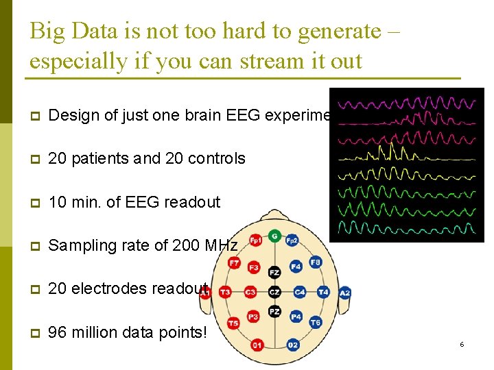
Big Data is not too hard to generate – especially if you can stream it out p Design of just one brain EEG experiment p 20 patients and 20 controls p 10 min. of EEG readout p Sampling rate of 200 MHz p 20 electrodes readout p 96 million data points! 6

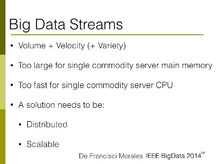
The Problem of Relentless Data Generation p Many organizations today produce an electronic record of essentially every transaction they are involved in. p This results in hundreds of millions of records being produced everyday. n E. g. In a single day Wal. Mart records 20 million sales transactions, Google handles 150 million searches, and AT&T produces 270 million call records. p Data rates of this level have significant consequences for data mining. n A few months’ worth data can easily add up to billions of records, and the entire history of transactions or 7 observations can be in hundreds of billions.

Concerns with mining “as usual” p Current algorithms for mining complex models from data (such as decision trees, set of association rules, outlier analysis) can not mine even a fraction of this data in useful time. p Mining a day’s worth of data can take more than a day of CPU time. n Data accumulates faster than it can be mined. n The fraction of the available data that we are able to mine in useful time is rapidly dwindling towards zero. p Overcoming this state of affairs requires a shift in our frame of mind from mining database to mining data 8

The Problem (Contd. ) p In the traditional data mining process, data loaded into a stable, infrequently–updated databases. n Mining it can take weeks or months. n Tradeoff between accuracy and speed. p The data mining system should be continuously on. n Processing records must take place at the speed they arrive. n Incorporating them into the model it is building even if it never sees them again. 9

Big Data Analytics 10

What is Big Data Analytics? Analytical abilities that are specifically required to address such characteristics of data (input) and results (output) as: p Large volume – storage, access p High velocity – data in motion, time-changing processes p Unusual variety – structured, unstructured (text, sound, pictures) p Uncertain veracity – data reliability if not sampled or designed p Issues of security, privacy and ethics – unintended data sources p High-dimensionality – curse of dimensionality 11 p Incidental endogenity – spurious correlations

The power of Big Data Mining p p Narrative Science can not only produce a story from given data by “joining the dots”, but can actually conceive a story from data even when no dots are given to it (i. e. when humans are clueless). Pred. Pol seeks to predict criminal activity patterns before any crime has occurred, which can lead to proactive rather than reactive policing. Google Hummingbird tries to search based on contexts and semantics of an input sentence, and not merely the words in it. IBM Watson improves on the subjective task of disease diagnosis – but can it do better than human experts, say, 12 on Autism spectrum disorders?

Stream Data Analysis 13

14

15

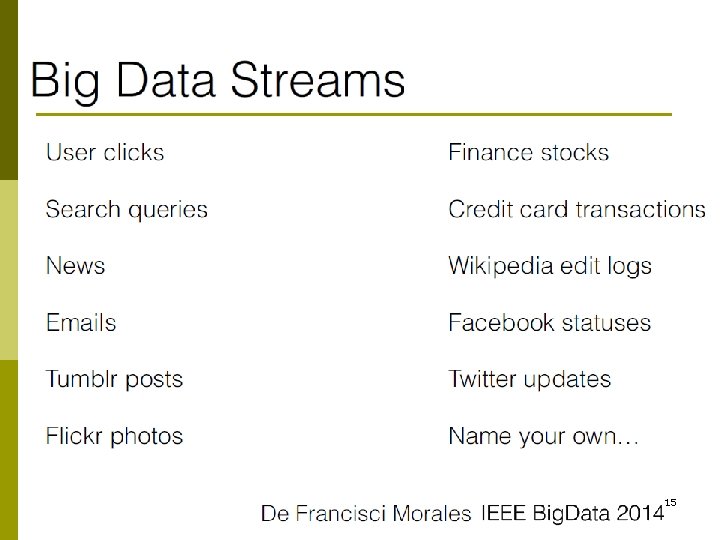
Background of Stream Data Analysis p p Typical statistical and data mining methods (e. g. , clustering, regression, classification and frequent pattern mining) work with “static” data sets, meaning that the complete data set is available as a whole to perform all necessary computations on it. Well known traditional methods like k-means / PAM clustering, linear regression, decision tree based classification and the APRIORI algorithm to find frequent itemsets generally scan the complete data set repeatedly to produce their results. However, in recent years more and more applications need to work with data which are not static, but are the result of a continuous data generation process (“data in motion”) which is likely to evolve (and change) over time. Some examples are web click-stream data, computer network monitoring data, telecommunication connection data, news RSS feeds, readings from sensor networks (such as in health and 16 environmental monitoring) and stock quotes.

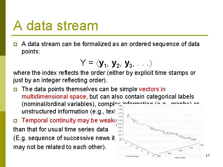
A data stream p A data stream can be formalized as an ordered sequence of data points: Y = y 1, y 2, y 3, . . . where the index reflects the order (either by explicit time stamps or just by an integer reflecting order). p The data points themselves can be simple vectors in multidimensional space, but can also contain categorical labels (nominal/ordinal variables), complex information (e. g. , graphs) or unstructured information (e. g. , text or snapshots). p Temporal continuity may be weaker than that for usual time series data (E. g. sequence of successive news items may not be related to each other). 17

Stream characteristics The characteristic of continually arriving data points introduces an important property of data streams which also poses the greatest challenge: the size of a data stream is potentially unbounded. This leads to the following requirements for data stream processing algorithms: p p Bounded storage: The algorithm can only store a very limited amount of data to summarize the data stream. Single pass: The incoming data points cannot be permanently stored and need to be processed at once in the arriving order. Real-time: The algorithm has to process data points on average at least as fast as the data is arriving. Concept drift: The algorithm has to be able to deal with a data generating process which evolves over time (e. g. , distributions change or new structure in the data appears). 18

Design Criteria for mining High Speed Data Streams p A system capable of overcoming these High-velocity problem needs to meet a number of stringent design criteria / or requirements: 1. 2. 3. 4. It must be able to build a model using at most one scan of the data. It must use only a fixed amount of main memory. It must require small constant time per record. It must make a usable model available at any point in time, as opposed to only when it is done processing the data, since it may never be done processing. n Ideally, it should produce a model that is equivalent to the one that would be obtained by the corresponding ordinary database mining algorithm, operating without the above constraints. n When the data-generating phenomenon is changing over time, the model at any time should be up-to-date. 19

Stream data resources in R and other platforms 20

R Distributed computing p p p With the development of Hadoop, distributed computing for statistical frameworks to solve large scale computational problems have become very popular. Hadoop. Streaming (Rosenberg 2012) is available to use R map and reduce scripts within the Hadoop framework. Hadoop. Streaming is used for batch processing. However, contrary to the word streaming in its name, Hadoop-Streaming does not support data streams. As with Hadoop itself, (Streaming in the name refers only to the internal usage of pipelines for “streaming” the input and output between the Hadoop framework and the used R scripts). A distributed framework for real-time computation is Storm (Apache). Storm builds on the idea of constructing a computing topology from spouts (data sources) and bolts (computational units). RStorm (Kaptein 2013) implements a simple, non-distributed version of Storm with multi-language capacity. 21

R: Stream Data sources p p p Random numbers are typically created as a stream (see e. g. , rstream (Leydold 2012) and rlecuyer (Sevcikova and Rossini 2012)). Financial data can be obtained via packages like quantmod (Ryan 2013). Intra-day price and trading volume can be considered a data stream. For Twitter, a popular micro-blogging service, packages like stream. R (Barbera 2014) and twitte. R (Gentry 2013) provide interfaces to retrieve life Twitter feeds. 22

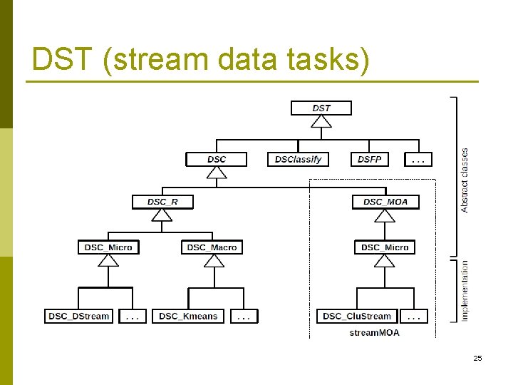
R stream package p p p 1. 2. The stream framework provides a R-based alternative to MOA which seamlessly integrates with the extensive existing R infrastructure. Since R can interface code written in a whole set of different programming languages (e. g. , C/C++, Java, Python), data stream mining algorithms in any of these languages can be easily integrated into stream. The stream framework consists of two main components: Data Stream Data (DSD) which manages or creates a data stream, and Data Stream Task (DST) which performs a data stream mining task. 23

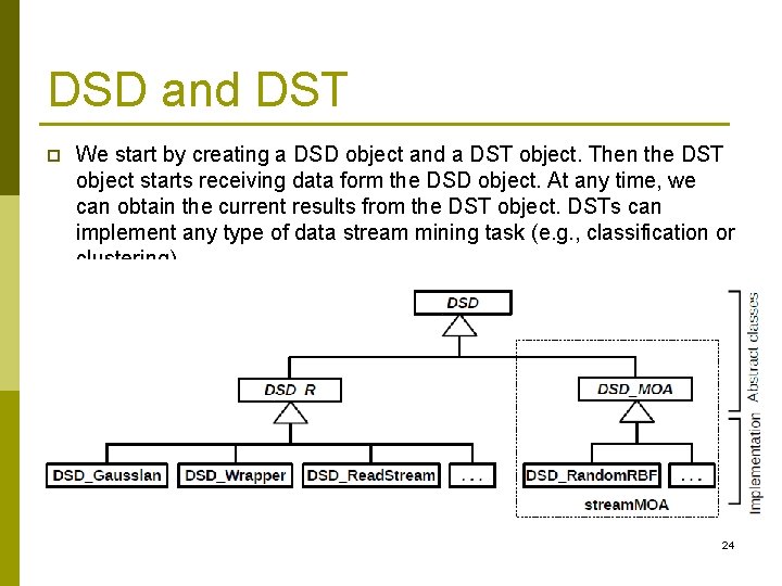
DSD and DST p We start by creating a DSD object and a DST object. Then the DST object starts receiving data form the DSD object. At any time, we can obtain the current results from the DST object. DSTs can implement any type of data stream mining task (e. g. , classification or clustering). 24

DST (stream data tasks) 25

Massive Online Analysis (MOA) “Online” analysis refers to learning that happens upon entry of each new data point. So it acts in a dynamic “then and there” manner. p MOA is a framework implemented in Java for stream classification, regression and clustering (Bifet, Holmes, Kirkby, and Pfahringer 2010). p It was the first experimental framework to provide easy access to multiple data stream mining algorithms, as well as tools to generate data streams that can be used to measure and compare the performance of different ML algorithms. p Like WEKA (Witten and Frank 2005), a popular collection of machine learning algorithms, MOA is also developed by the University of Waikato and its interface and workflow are similar to those of WEKA. 26 p The workflow in MOA consists of three main steps: p Selection of the data stream model (also called data feeds). p

MOA (cont’d) p p p Similar to WEKA, MOA uses a very appealing graphical user interface. Classification results are shown as text, while clustering results have a visualization component that shows both the evolution of the clustering (in two dimensions) and various performance metrics over time. MOA is currently the most complete framework for data stream clustering research. MOA’s advantages are that it interfaces with WEKA, provides already a set of data stream classification and clustering algorithms and it has a clear Java interface to add new algorithms or use the existing algorithms in other applications. A drawback of MOA and the other frameworks for R users is that for all (but very simple) experiments custom Java code has to be written. 27

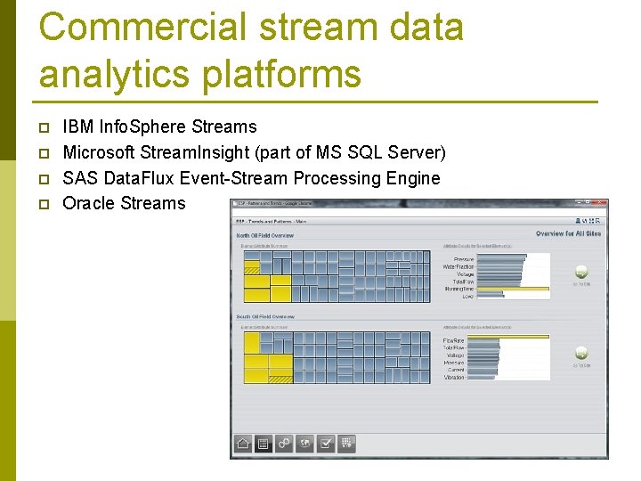
Commercial stream data analytics platforms p p IBM Info. Sphere Streams Microsoft Stream. Insight (part of MS SQL Server) SAS Data. Flux Event-Stream Processing Engine Oracle Streams 28

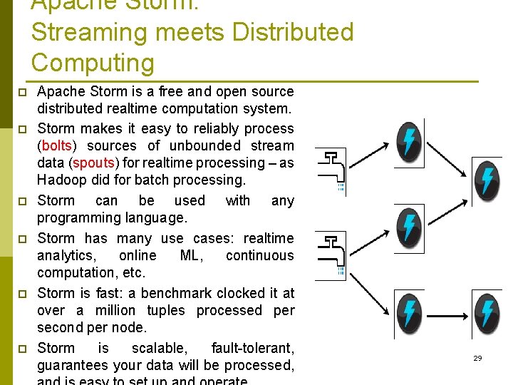
Apache Storm: Streaming meets Distributed Computing p p p Apache Storm is a free and open source distributed realtime computation system. Storm makes it easy to reliably process (bolts) sources of unbounded stream data (spouts) for realtime processing – as Hadoop did for batch processing. Storm can be used with any programming language. Storm has many use cases: realtime analytics, online ML, continuous computation, etc. Storm is fast: a benchmark clocked it at over a million tuples processed per second per node. Storm is scalable, fault-tolerant, guarantees your data will be processed, 29

Apache Spark (Streaming) p p p Apache Spark is an in-memory distributed data analysis platform-- primarily targeted at speeding up batch analysis jobs, iterative machine learning jobs, interactive query and graph processing. One of Spark's primary distinctions is its use of RDDs or Resilient Distributed Datasets. RDDs are great for pipelining parallel operators for computation and are, by definition, immutable, which allows Spark a unique form of fault tolerance based on lineage information. If you are interested in, say, executing a Hadoop Map. Reduce job much faster, Spark is a great option (although memory requirements must be considered). Since Spark's RDDs are inherently immutable, Spark 30 Streaming implements a method for "batching" incoming

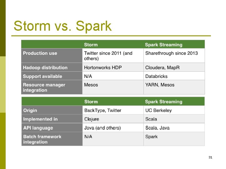
Storm vs. Spark 31

Copyright Note: This presentation is based on the following papers: 1. Mining High-Speed Data Streams, P. Domingos and Geoff Hulten. Proceedings of the Sixth International Conference on Knowledge Discovery and Data Mining. ACM Press. pp. 7180, 2000. 2. A General Framework for Mining Massive Data Streams, Geoff Hulten (short paper). Journal of Computational and Graphical Statistics, 12, 2003. 3. Mining time-changing data streams. G. Hulten et al. Proceedings of the seventh ACM SIGKDD international conference on Knowledge discovery and data mining. ACM Press, NY, pp. 97 -106, 2001. 32 4. Introduction to stream: An Extensible Framework for Data

Stream data clustering 33

Data Stream Clustering p p Clustering, the assignment of data points to (typically k) groups such that points within each group are more similar to each other than to points in different groups, is a very basic unsupervised data mining task. For static data sets methods like k-means, k-medians, PAM, hierarchical clustering and density-based methods have been developed among others. Many of these methods are available in tools like R, however, the standard algorithms need access to all data points and typically iterate over the data multiple times. This requirement makes these algorithms unsuitable for data streams and led to the development of data stream clustering algorithms. Over the last 10 years many algorithms for clustering data streams have been proposed. Most data stream clustering algorithms that deal with the problems of unbounded stream size, and the requirements 34 for real-time processing in a single pass, often use the two-stage

Step 1 p p Online: Summarize the data using a set of k′ micro-clusters organized in a space- efficient data structure which also enables fast look-up. Microclusters were introduced for Clu. Stream by Aggarwal et al. (2003) based on the idea of cluster features developed for clustering large data sets with the BIRCH algorithm. Micro-clusters are representatives for sets of similar data points and are created using a single pass over the data (typically in real time when the data stream arrives). Micro-clusters are typically represented by cluster centers and additional statistics such as weight (local density) and dispersion (variance). The individual data-points are then let gone – a truly unique situation in Statistics. Each new data point is assigned to its closest (in terms of a similarity function) micro-cluster center. Some algorithms use a grid instead and micro-clusters are represented by non-empty grid cells (e. g. , D-Stream by 35 Tu and Chen (2009)).

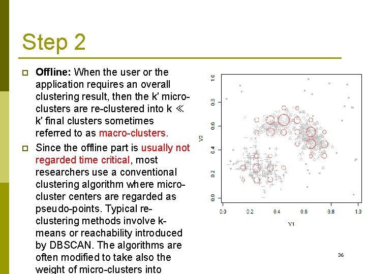
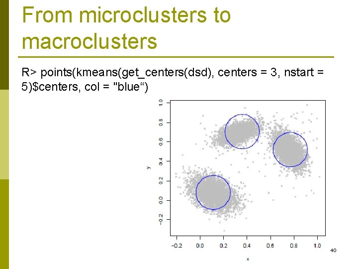
Step 2 p p Offline: When the user or the application requires an overall clustering result, then the k′ microclusters are re-clustered into k ≪ k′ final clusters sometimes referred to as macro-clusters. Since the offline part is usually not regarded time critical, most researchers use a conventional clustering algorithm where microcluster centers are regarded as pseudo-points. Typical reclustering methods involve kmeans or reachability introduced by DBSCAN. The algorithms are often modified to take also the weight of micro-clusters into 36

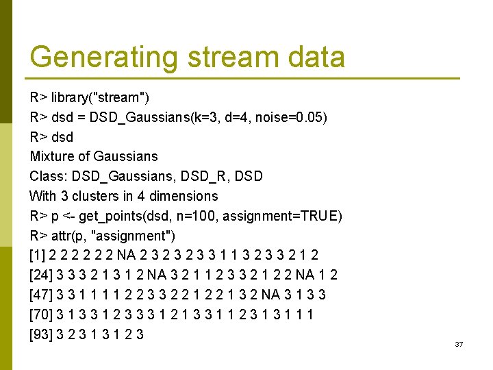
Generating stream data R> library("stream") R> dsd = DSD_Gaussians(k=3, d=4, noise=0. 05) R> dsd Mixture of Gaussians Class: DSD_Gaussians, DSD_R, DSD With 3 clusters in 4 dimensions R> p <- get_points(dsd, n=100, assignment=TRUE) R> attr(p, "assignment") [1] 2 2 2 NA 2 3 2 3 3 1 1 3 2 3 3 2 1 2 [24] 3 3 3 2 1 3 1 2 NA 3 2 1 1 2 3 3 2 1 2 2 NA 1 2 [47] 3 3 1 1 2 2 3 3 2 2 1 3 2 NA 3 1 3 3 [70] 3 1 3 3 1 2 3 3 3 1 2 1 3 3 1 1 2 3 1 1 1 [93] 3 2 3 1 2 3 37

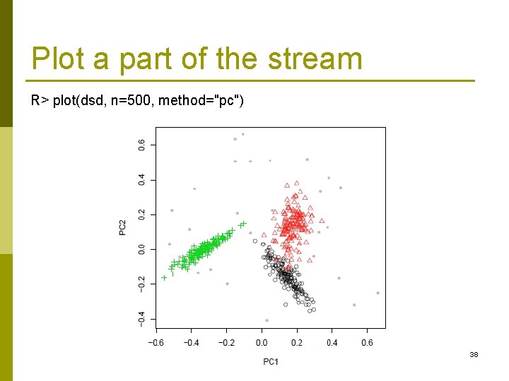
Plot a part of the stream R> plot(dsd, n=500, method="pc") 38

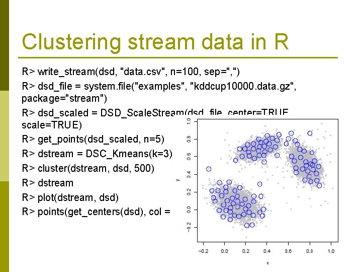
Clustering stream data in R R> write_stream(dsd, "data. csv", n=100, sep=", ") R> dsd_file = system. file("examples", "kddcup 10000. data. gz", package="stream") R> dsd_scaled = DSD_Scale. Stream(dsd_file, center=TRUE, scale=TRUE) R> get_points(dsd_scaled, n=5) R> dstream = DSC_Kmeans(k=3) R> cluster(dstream, dsd, 500) R> dstream R> plot(dstream, dsd) R> points(get_centers(dsd), col = "blue“) 39

From microclusters to macroclusters R> points(kmeans(get_centers(dsd), centers = 3, nstart = 5)$centers, col = "blue“) 40

Concept drift data streams 41

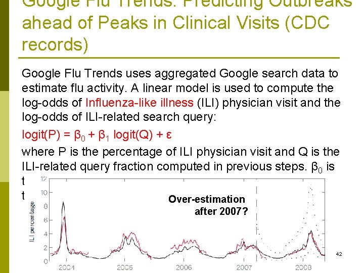
Google Flu Trends: Predicting Outbreaks ahead of Peaks in Clinical Visits (CDC records) Google Flu Trends uses aggregated Google search data to estimate flu activity. A linear model is used to compute the log-odds of Influenza-like illness (ILI) physician visit and the log-odds of ILI-related search query: logit(P) = β 0 + β 1 logit(Q) + ε where P is the percentage of ILI physician visit and Q is the ILI-related query fraction computed in previous steps. β 0 is the intercept and β 1 is the coefficient, while ε is the error term. Over-estimation after 2007? 42

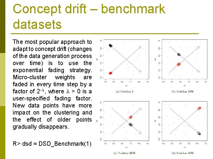
Concept drift – benchmark datasets The most popular approach to adapt to concept drift (changes of the data generation process over time) is to use the exponential fading strategy. Micro-cluster weights are faded in every time step by a factor of 2− , where > 0 is a user-specified fading factor. New data points have more impact on the clustering and the effect of older points gradually disappears. R> dsd = DSD_Benchmark(1) 43

Concept Drift in Economics Macroeconomic forecasts and financial time series are also subjects to data stream mining. The data in those applications is drifting primary due to a large number of factors that are not included in the model. p The publicly known information about companies can form only a small part of attributes needed to properly model financial forecasts as a stationary problem. That is why the main source of drift is hidden context. p 44

Concept Drift in Finance Bankruptcy prediction or individual credit scoring is typically considered to be a stationary problem. p Again, there is drift due to hidden context. The decisions that need to be made by the system are based on fragmentary information. p The need for different models for bankruptcy prediction under different economic conditions was acknowledged, but the need for models to be able to deal with non-stationarity has been rarely researched. p 45

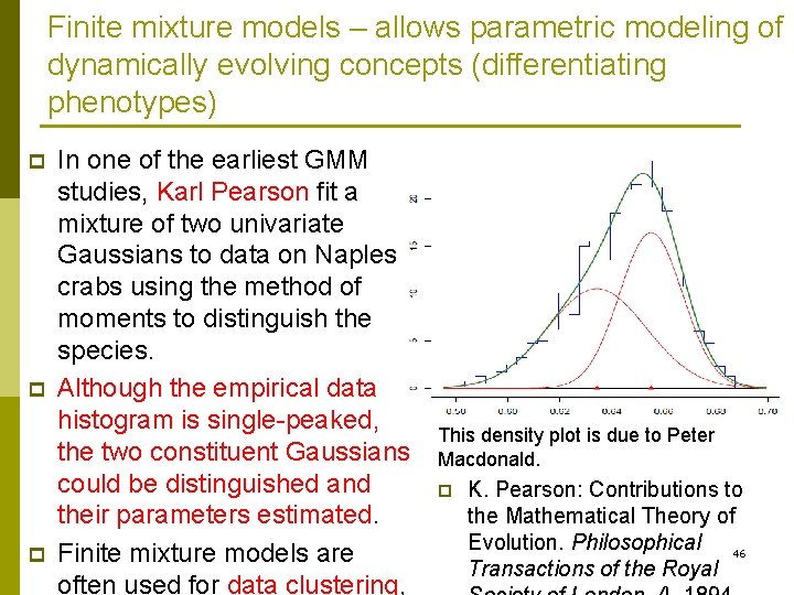
Finite mixture models – allows parametric modeling of dynamically evolving concepts (differentiating phenotypes) p p p In one of the earliest GMM studies, Karl Pearson fit a mixture of two univariate Gaussians to data on Naples crabs using the method of moments to distinguish the species. Although the empirical data histogram is single-peaked, the two constituent Gaussians could be distinguished and their parameters estimated. Finite mixture models are often used for data clustering, This density plot is due to Peter Macdonald. p K. Pearson: Contributions to the Mathematical Theory of Evolution. Philosophical 46 Transactions of the Royal

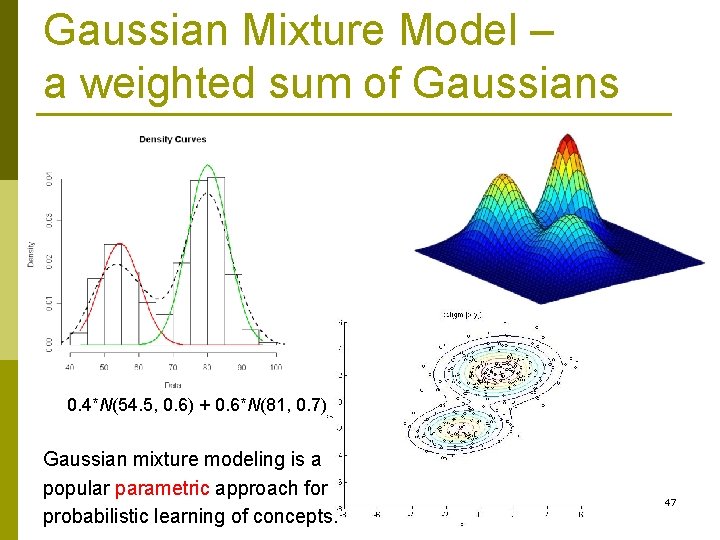
Gaussian Mixture Model – a weighted sum of Gaussians 0. 4*N(54. 5, 0. 6) + 0. 6*N(81, 0. 7) Gaussian mixture modeling is a popular parametric approach for probabilistic learning of concepts. 47

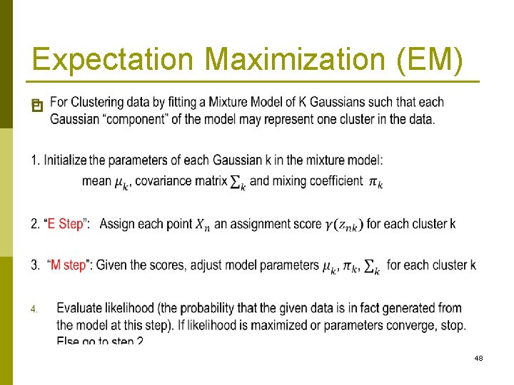
Expectation Maximization (EM) p 48

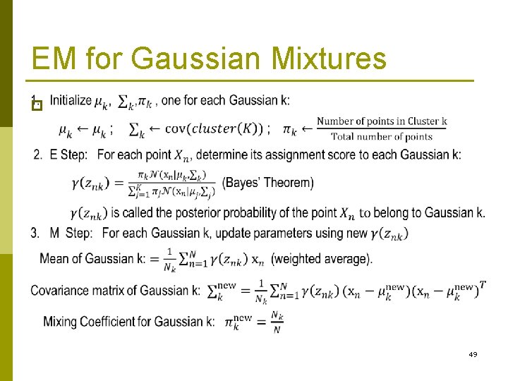
EM for Gaussian Mixtures p 49

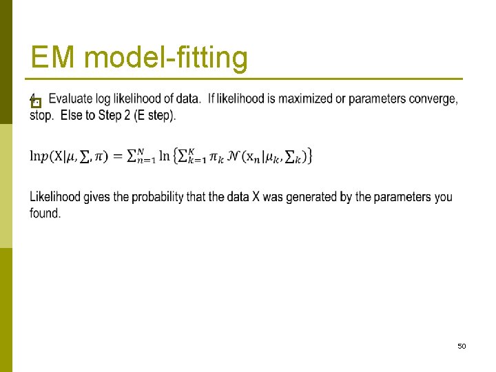
EM model-fitting p 50

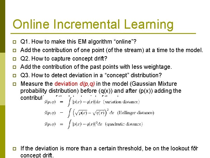
Online Incremental Learning p p p p Q 1. How to make this EM algorithm “online”? Add the contribution of one point (of the stream) at a time to the model. Q 2. How to capture concept drift? Add the contribution of the past points with less weightage. Q 3. How to detect deviation in a “concept” distribution? Measure the deviation d(p, q) in the model (Gaussian Mixture probability distribution) before (q(x)) and after (p(x)) adding the contribution of the latest point of the stream. 51 If the deviation is more than a certain threshold, be on the lookout for concept drift.

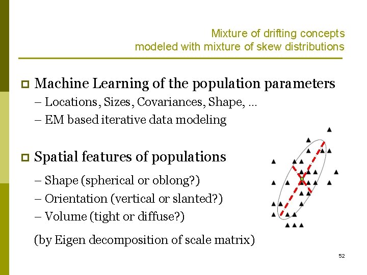
Mixture of drifting concepts modeled with mixture of skew distributions p Machine Learning of the population parameters – Locations, Sizes, Covariances, Shape, … – EM based iterative data modeling p Spatial features of populations – Shape (spherical or oblong? ) – Orientation (vertical or slanted? ) – Volume (tight or diffuse? ) (by Eigen decomposition of scale matrix) 52

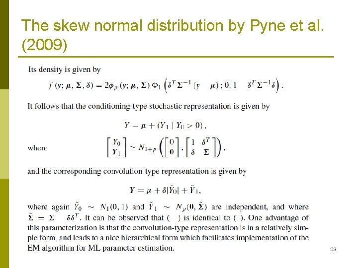
The skew normal distribution by Pyne et al. (2009) 53

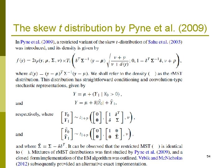
The skew t distribution by Pyne et al. (2009) 54

Stream data Classification 55

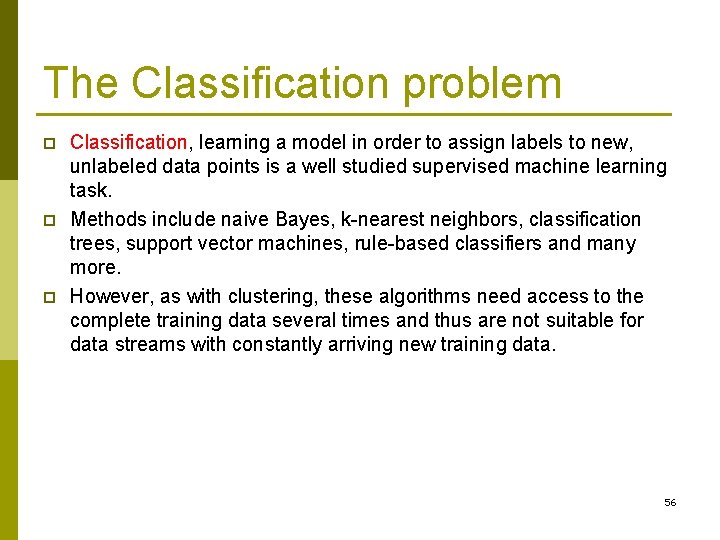
The Classification problem p p p Classification, learning a model in order to assign labels to new, unlabeled data points is a well studied supervised machine learning task. Methods include naive Bayes, k-nearest neighbors, classification trees, support vector machines, rule-based classifiers and many more. However, as with clustering, these algorithms need access to the complete training data several times and thus are not suitable for data streams with constantly arriving new training data. 56

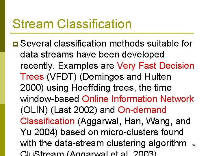
Stream Classification p Several classification methods suitable for data streams have been developed recently. Examples are Very Fast Decision Trees (VFDT) (Domingos and Hulten 2000) using Hoeffding trees, the time window-based Online Information Network (OLIN) (Last 2002) and On-demand Classification (Aggarwal, Han, Wang, and Yu 2004) based on micro-clusters found with the data-stream clustering algorithm 57

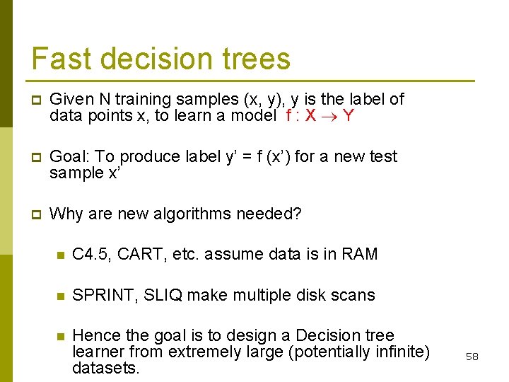
Fast decision trees p Given N training samples (x, y), y is the label of data points x, to learn a model f : X Y p Goal: To produce label y’ = f (x’) for a new test sample x’ p Why are new algorithms needed? n C 4. 5, CART, etc. assume data is in RAM n SPRINT, SLIQ make multiple disk scans n Hence the goal is to design a Decision tree learner from extremely large (potentially infinite) datasets. 58

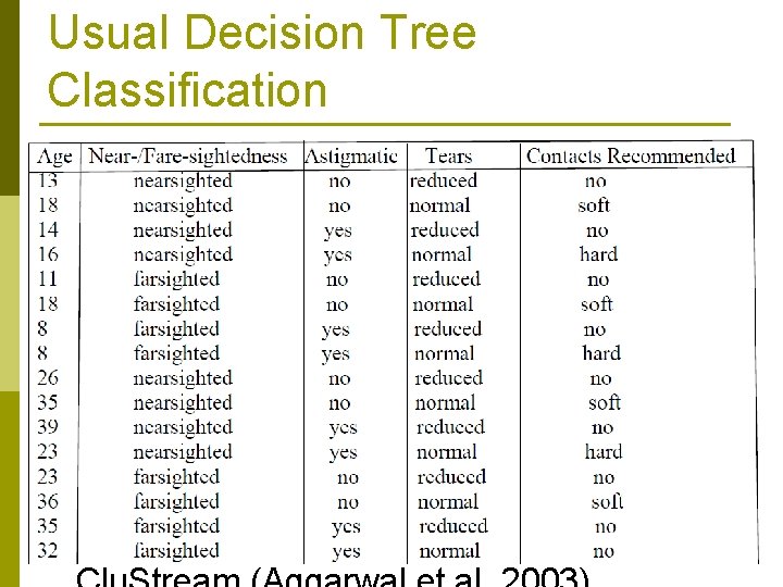
Usual Decision Tree Classification p Several classification methods suitable for data streams have been developed recently. Examples are Very Fast Decision Trees (VFDT) (Domingos and Hulten 2000) using Hoeffding trees, the time window-based Online Information Network (OLIN) (Last 2002) and On-demand Classification (Aggarwal, Han, Wang, and Yu 2004) based on micro-clusters found with the data-stream clustering algorithm 59

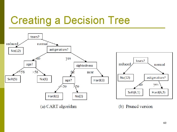
Creating a Decision Tree 60

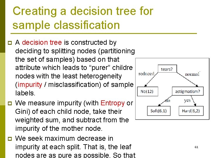
Creating a decision tree for sample classification p p p A decision tree is constructed by deciding to splitting nodes (partitioning the set of samples) based on that attribute which leads to “purer” children nodes with the least heterogeneity (impurity / misclassification) of sample labels. We measure impurity (with Entropy or Gini) of each child node, take their weighted sum, and subtract from the impurity of the mother node. We seek maximum decrease in impurity at each split. That is, the leaf nodes are as pure as possible. So that 61

Can we create a good enough decision tree by training a node with only a small # of samples? p p A decision tree selects a data attribute at each node, and uses it to split the dataset at that node into 2 parts. The “goodness” of a split is measured by a resulting decrease in the uncertainty of class membership of the 2 split subsets while moving down the tree from a parent node to its 2 children nodes. Hoeffding bound ensures that it is unlikely that a split at a given node, determined by reading only a sample of certain size (N points), will be much worse than a split at the same node which is determined by reading the full dataset as is usually done for creating a conventional decision tree. The probability that the Hoeffding and conventional tree 62

How does VFDT work? The VFDT method (Domingos & Hulten, 2000) is based on the principle of the Hoeffding tree. A Hoeffding tree is constructed not with the full (highvolume high-velocity) stream but with the use of random sampling on static data. p The idea is to determine a random sample of sufficient size so that the tree constructed on the sample is approximately the same as that constructed on the entire data set. The Hoeffding bound is used to ensure that the decision tree on the sub-sampled tree would make the same decisions or “split”s as an usual tree that is created p 63

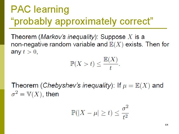
PAC learning “probably approximately correct” 64

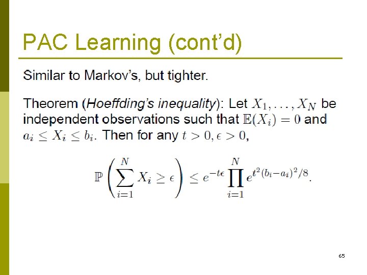
PAC Learning (cont’d) 65

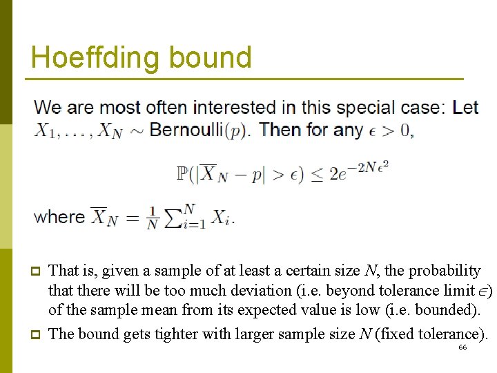
Hoeffding bound p p That is, given a sample of at least a certain size N, the probability that there will be too much deviation (i. e. beyond tolerance limit ) of the sample mean from its expected value is low (i. e. bounded). The bound gets tighter with larger sample size N (fixed tolerance). 66

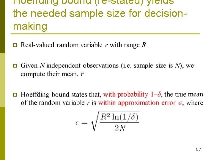
Hoeffding bound (re-stated) yields the needed sample size for decisionmaking 67

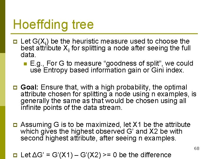
Hoeffding tree p Let G(Xi) be the heuristic measure used to choose the best attribute Xi for splitting a node after seeing the full data. n E. g. , For G to measure “goodness of split”, we could use Entropy based information gain or Gini index. p Goal: Ensure that, with a high probability, the optimal attribute chosen for splitting a node using n examples, is generally the same as that would be chosen using all infinite points of the data stream. p Assuming G is to be maximized, let X 1 be the attribute which gives the highest observed G’ and X 2 be with second highest attribute, after seeing n examples. 68 p Let ΔG’ = G’(X 1) – G’(X 2) >= 0 be the difference

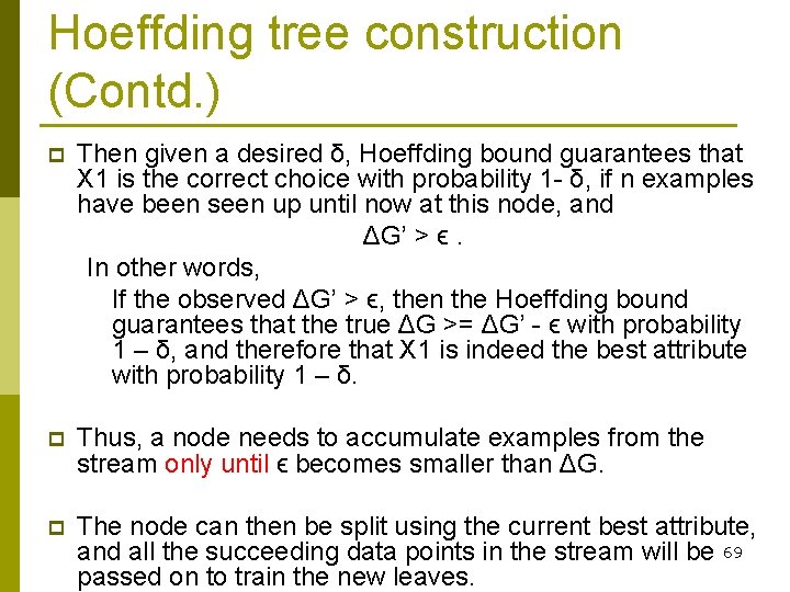
Hoeffding tree construction (Contd. ) p Then given a desired δ, Hoeffding bound guarantees that X 1 is the correct choice with probability 1 - δ, if n examples have been seen up until now at this node, and ΔG’ > ϵ. In other words, If the observed ΔG’ > ϵ, then the Hoeffding bound guarantees that the true ΔG >= ΔG’ - ϵ with probability 1 – δ, and therefore that X 1 is indeed the best attribute with probability 1 – δ. p Thus, a node needs to accumulate examples from the stream only until ϵ becomes smaller than ΔG. p The node can then be split using the current best attribute, and all the succeeding data points in the stream will be 69 passed on to train the new leaves.

Stream Anomaly Detection 70

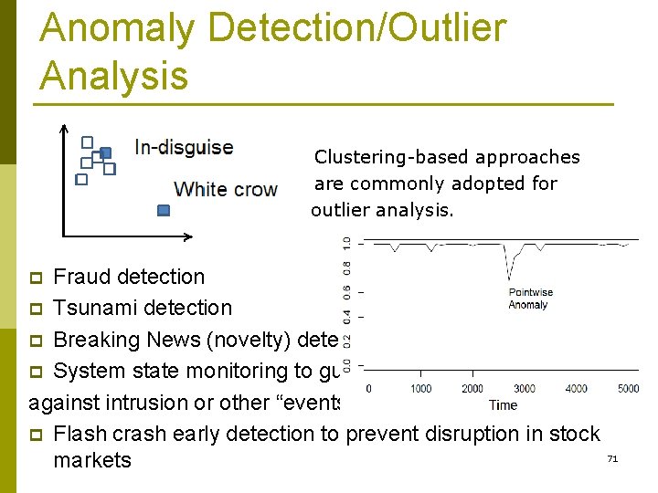
Anomaly Detection/Outlier Analysis Clustering-based approaches are commonly adopted for outlier analysis. Fraud detection p Tsunami detection p Breaking News (novelty) detection p System state monitoring to guard against intrusion or other “events” p Flash crash early detection to prevent disruption in stock markets p 71

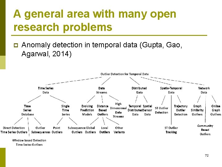
A general area with many open research problems p Anomaly detection in temporal data (Gupta, Gao, Agarwal, 2014) 72

Stream data Applications: Health Analytics and Disease Modeling Lab 73

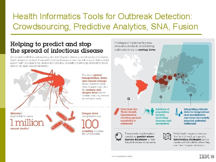
Health Informatics Tools for Outbreak Detection: Crowdsourcing, Predictive Analytics, SNA, Fusion 74

Various data stream sources incorporated in Public Health Analytics & Outbreak Detection p p p p Social Networks Census and demographics studies Environmental monitoring and sensor networks Electronic health records Monitoring of lifestyle parameters Media reports and trends Environmental and occupational exposures Civil unrest, riot, war, migration, displacement spatiotemporal data Therefore, it calls for design of – p Integrative frameworks with hierarchical models with 75

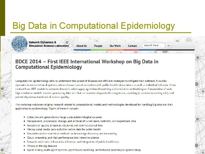
Big Data in Computational Epidemiology 76

Engaging the BD Community Past few months: p National Big Data Workshop, Hyderabad (Aug. 2014) p ACM Big. LS 2014, Newport Beach, CA (Sept. 2014) p IEEE Big. Data 2014, Washington DC (Oct. 2014) p Big. LSW 2014, C-DAC, Bangalore (Dec. 2014) p DST Curriculum Design for Big Data, Hyderabad (Mar. 2015) 77

78

Thank you for your kind attention Acknowledgement for funding Mo. S&PI, DST, DRDE, DBT New NIH funded Health Analytics and Disease Modeling Lab (Sept. 2015) IIPH Hyderabad 79

80

Deadline: Sept. 28, 2015 81