296 3 Algorithms in the Real World Linear

296. 3: Algorithms in the Real World Linear and Integer Programming III – Integer Programming • Applications • Algorithms 296. 3 Page 1

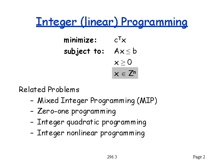
Integer (linear) Programming minimize: subject to: c Tx Ax ≤ b x≥ 0 x Zn Related Problems – Mixed Integer Programming (MIP) – Zero-one programming – Integer quadratic programming – Integer nonlinear programming 296. 3 Page 2

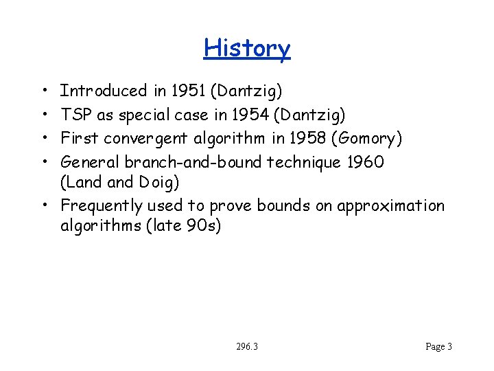
History • • Introduced in 1951 (Dantzig) TSP as special case in 1954 (Dantzig) First convergent algorithm in 1958 (Gomory) General branch-and-bound technique 1960 (Land Doig) • Frequently used to prove bounds on approximation algorithms (late 90 s) 296. 3 Page 3

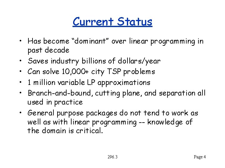
Current Status • Has become “dominant” over linear programming in past decade • Saves industry billions of dollars/year • Can solve 10, 000+ city TSP problems • 1 million variable LP approximations • Branch-and-bound, cutting plane, and separation all used in practice • General purpose packages do not tend to work as well as with linear programming -- knowledge of the domain is critical. 296. 3 Page 4

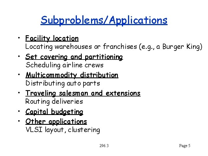
Subproblems/Applications • Facility location Locating warehouses or franchises (e. g. , a Burger King) • Set covering and partitioning Scheduling airline crews • Multicommodity distribution Distributing auto parts • Traveling salesman and extensions Routing deliveries • Capital budgeting • Other applications VLSI layout, clustering 296. 3 Page 5

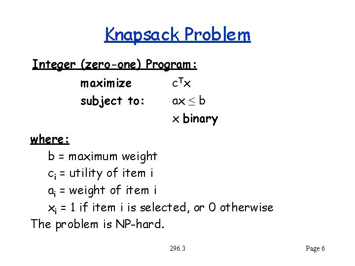
Knapsack Problem Integer (zero-one) Program: maximize subject to: c Tx ax ≤ b x binary where: b = maximum weight ci = utility of item i ai = weight of item i xi = 1 if item i is selected, or 0 otherwise The problem is NP-hard. 296. 3 Page 6

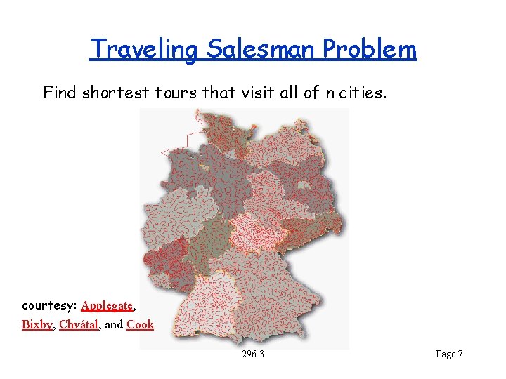
Traveling Salesman Problem Find shortest tours that visit all of n cities. courtesy: Applegate, Bixby, Chvátal, and Cook 296. 3 Page 7

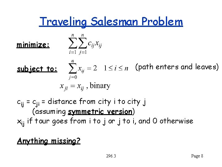
Traveling Salesman Problem minimize: (path enters and leaves) subject to: cij = cji = distance from city i to city j (assuming symmetric version) xij if tour goes from i to j or j to i, and 0 otherwise Anything missing? 296. 3 Page 8

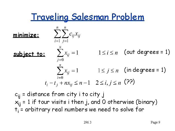
Traveling Salesman Problem minimize: (out degrees = 1) subject to: (in degrees = 1) (? ? ) cij = distance from city i to city j xij = 1 if tour visits i then j, and 0 otherwise (binary) ti = arbitrary real numbers we need to solve for 296. 3 Page 9

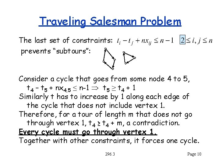
Traveling Salesman Problem The last set of constraints: prevents “subtours”: Consider a cycle that goes from some node 4 to 5, t 4 – t 5 + nx 4, 5 ≤ n-1 t 5 ≥ t 4 + 1 Similarly t has to increase by 1 along each edge of the cycle that does not include vertex 1. Therefore, for a tour of length m that does not go through vertex 1, t 4 ≥ t 4 + m, a contradiction. Every cycle must go through vertex 1. Together with other constraints, it forces one cycle. 296. 3 Page 10

Traveling Salesman Problem Many “Real World” applications based on the TSP. – They typically involve more involved constraints – Not just routing type problems. Consider a drug company with k drugs they can make at a lab. They can only make the drugs one at a time. The cost of converting the equipment from making drug i to drug j is cij Current best solutions are based on IP – Applegate, Bixby, et. al. , have solutions for more than 15 K cities in Germany > 150, 000 CPU hours (more info) – Involves “branch-and-bound” and “cutting planes” 296. 3 Page 11

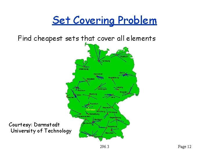
Set Covering Problem Find cheapest sets that cover all elements Courtesy: Darmstadt University of Technology 296. 3 Page 12

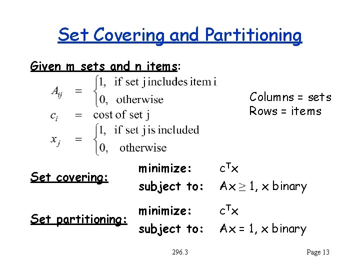
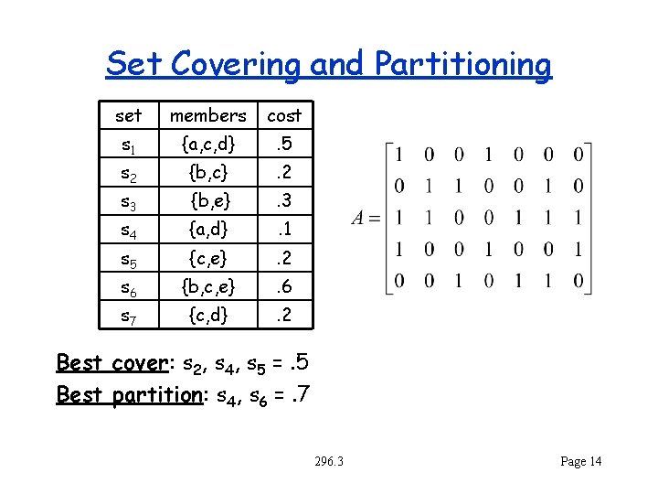
Set Covering and Partitioning Given m sets and n items: Columns = sets Rows = items minimize: subject to: c Tx Ax ≥ 1, x binary minimize: Set partitioning: subject to: c Tx Ax = 1, x binary Set covering: 296. 3 Page 13

Set Covering and Partitioning set members cost s 1 {a, c, d} . 5 s 2 {b, c} . 2 s 3 {b, e} . 3 s 4 {a, d} . 1 s 5 {c, e} . 2 s 6 {b, c, e} . 6 s 7 {c, d} . 2 Best cover: s 2, s 4, s 5 =. 5 Best partition: s 4, s 6 =. 7 296. 3 Page 14

Set Covering and Partitioning Applications: • Facility location. Each set is a facility (e. g. , warehouse, fire station, emergency response center). Each item is an area that needs to be covered • Crew scheduling. Each set is a route for a particular crew member (e. g. NYC->Pit->Atlanta->NYC). Each item is a flight that needs to be covered. 296. 3 Page 15

Constraints Expressible with IP Many constraints are expressible with integer programming: – logical constraints (e. g. , x implies not y) – k out of n – piecewise linear functions – … and many more 296. 3 Page 16

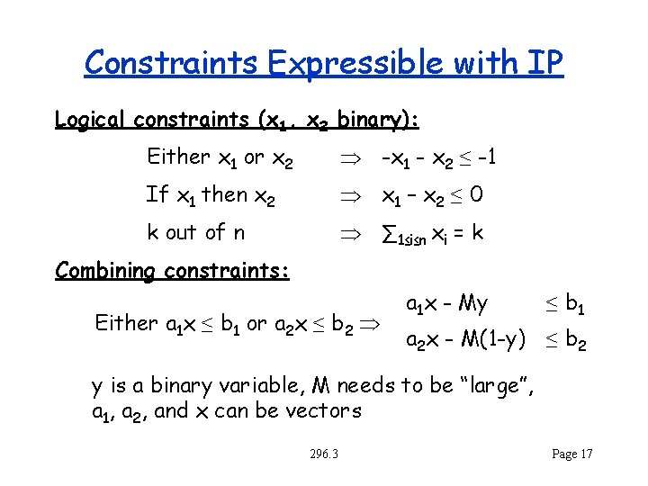
Constraints Expressible with IP Logical constraints (x 1, x 2 binary): Either x 1 or x 2 -x 1 - x 2 ≤ -1 If x 1 then x 2 x 1 – x 2 ≤ 0 k out of n ∑ 1≤i≤n xi = k Combining constraints: Either a 1 x ≤ b 1 or a 2 x ≤ b 2 a 1 x - My ≤ b 1 a 2 x - M(1 -y) ≤ b 2 y is a binary variable, M needs to be “large”, a 1, a 2, and x can be vectors 296. 3 Page 17

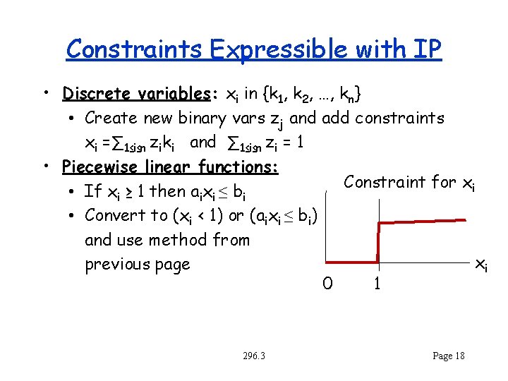
Constraints Expressible with IP • Discrete variables: xi in {k 1, k 2, …, kn} • Create new binary vars zj and add constraints xi =∑ 1≤i≤n ziki and ∑ 1≤i≤n zi = 1 • Piecewise linear functions: Constraint for xi • If xi ≥ 1 then aixi ≤ bi • Convert to (xi < 1) or (aixi ≤ bi) and use method from xi previous page 0 1 296. 3 Page 18

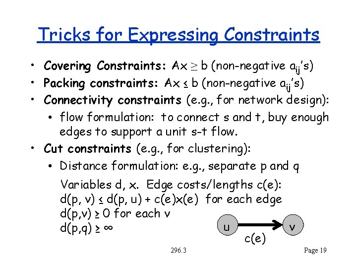
Tricks for Expressing Constraints • Covering Constraints: Ax ≥ b (non-negative aij’s) • Packing constraints: Ax ≤ b (non-negative aij’s) • Connectivity constraints (e. g. , for network design): • flow formulation: to connect s and t, buy enough edges to support a unit s-t flow. • Cut constraints (e. g. , for clustering): • Distance formulation: e. g. , separate p and q Variables d, x. Edge costs/lengths c(e): d(p, v) ≤ d(p, u) + c(e)x(e) for each edge d(p, v) ≥ 0 for each v u v d(p, q) ≥ ∞ c(e) 296. 3 Page 19

Algorithms 1. Use a linear program – round to integer solution (what if not feasible? ) 2. Search – Branch and bound (integer ranges) – Implicit (0 -1 variables) 3. Cutting planes – Many variants 296. 3 Page 20

Important Properties • LP solution is an upper bound on IP solution (assuming maximization) • If LP is infeasible then IP is infeasible • If LP solution is integral (all variables have integer values), then it is the IP solution. 296. 3 Page 21

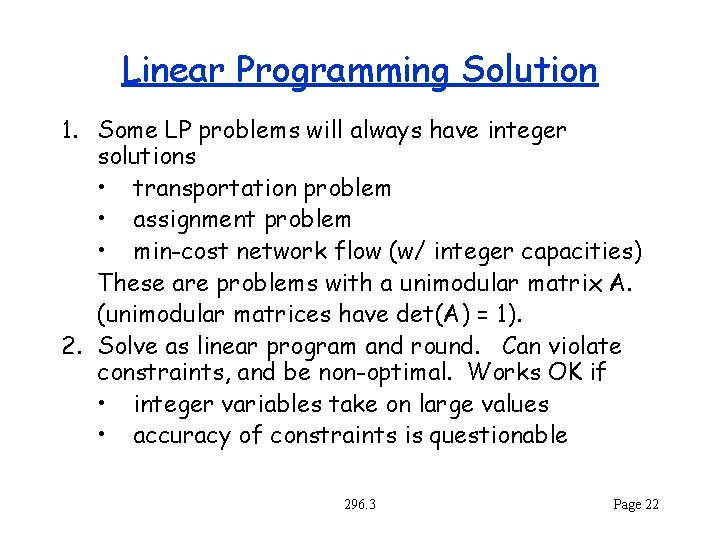
Linear Programming Solution 1. Some LP problems will always have integer solutions • transportation problem • assignment problem • min-cost network flow (w/ integer capacities) These are problems with a unimodular matrix A. (unimodular matrices have det(A) = 1). 2. Solve as linear program and round. Can violate constraints, and be non-optimal. Works OK if • integer variables take on large values • accuracy of constraints is questionable 296. 3 Page 22

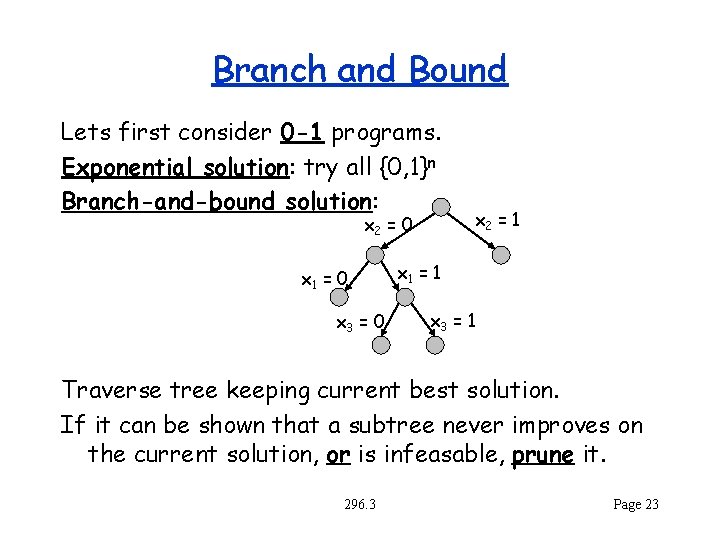
Branch and Bound Lets first consider 0 -1 programs. Exponential solution: try all {0, 1}n Branch-and-bound solution: x 2 = 0 x 1 = 0 x 3 = 0 x 2 = 1 x 1 = 1 x 3 = 1 Traverse tree keeping current best solution. If it can be shown that a subtree never improves on the current solution, or is infeasable, prune it. 296. 3 Page 23

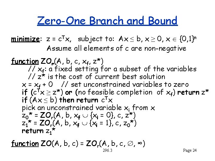
Zero-One Branch and Bound minimize: z = c. Tx, subject to: Ax ≤ b, x ≥ 0, x {0, 1}n Assume all elements of c are non-negative function ZOr(A, b, c, xf, z*) // xf: a fixed setting for a subset of the variables // z* is the cost of current best solution x = xf + 0 // set unconstrained variables to zero if (c. Tx ≥ z*) or (no feasible completion of xf) return z* if (Ax ≤ b) then return c. Tx pick an unconstrained variable xi from x z 0* = ZOr(A, b, xf {xi = 0}, c, z*) z 1* = ZOr(A, b, xf {xi = 1}, c, z 0*) return z 1* function ZO(A, b, c) = ZOr(A, b, c, Æ, ∞) 296. 3 Page 24

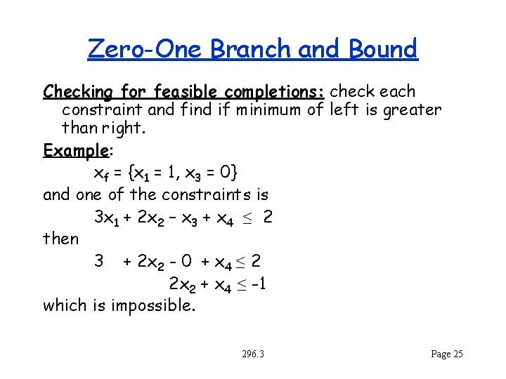
Zero-One Branch and Bound Checking for feasible completions: check each constraint and find if minimum of left is greater than right. Example: xf = {x 1 = 1, x 3 = 0} and one of the constraints is 3 x 1 + 2 x 2 – x 3 + x 4 ≤ 2 then 3 + 2 x 2 - 0 + x 4 ≤ 2 2 x 2 + x 4 ≤ -1 which is impossible. 296. 3 Page 25

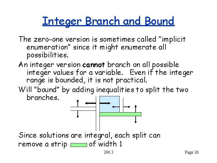
Integer Branch and Bound The zero-one version is sometimes called “implicit enumeration” since it might enumerate all possibilities. An integer version cannot branch on all possible integer values for a variable. Even if the integer range is bounded, it is not practical. Will “bound” by adding inequalities to split the two branches. Since solutions are integral, each split can remove a strip of width 1 296. 3 Page 26

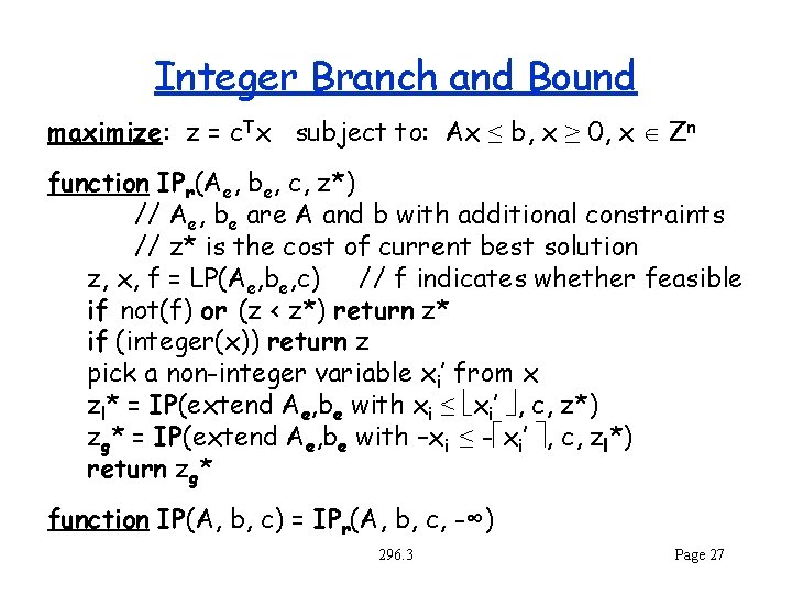
Integer Branch and Bound maximize: z = c. Tx subject to: Ax ≤ b, x ≥ 0, x Zn function IPr(Ae, be, c, z*) // Ae, be are A and b with additional constraints // z* is the cost of current best solution z, x, f = LP(Ae, be, c) // f indicates whether feasible if not(f) or (z < z*) return z* if (integer(x)) return z pick a non-integer variable xi’ from x zl* = IP(extend Ae, be with xi ≤ xi’ , c, z*) zg* = IP(extend Ae, be with –xi ≤ - xi’ , c, zl*) return zg* function IP(A, b, c) = IPr(A, b, c, -∞) 296. 3 Page 27

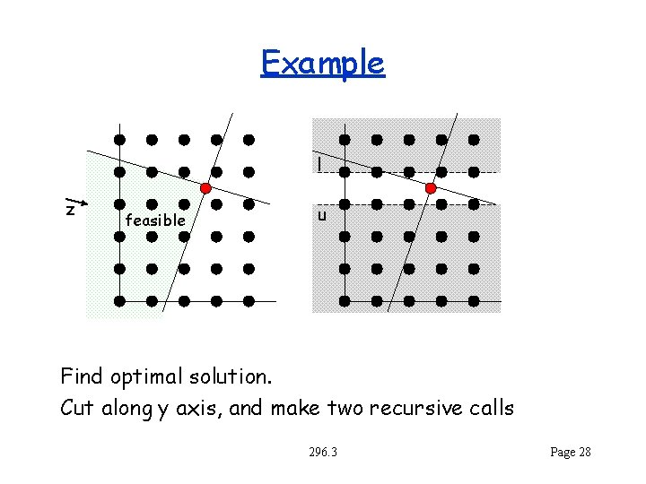
Example l z feasible u Find optimal solution. Cut along y axis, and make two recursive calls 296. 3 Page 28

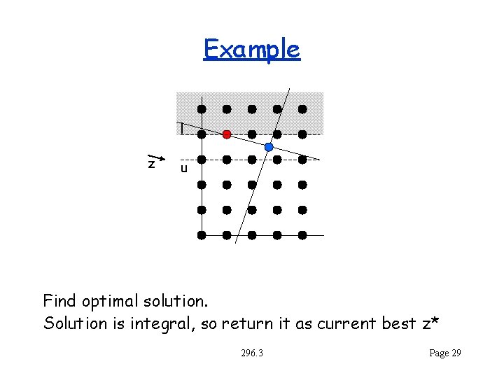
Example l z u Find optimal solution. Solution is integral, so return it as current best z* 296. 3 Page 29

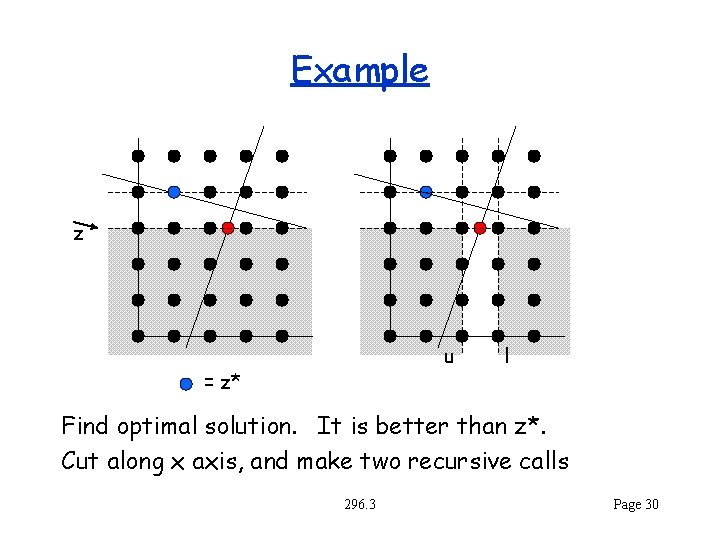
Example z u = z* l Find optimal solution. It is better than z*. Cut along x axis, and make two recursive calls 296. 3 Page 30

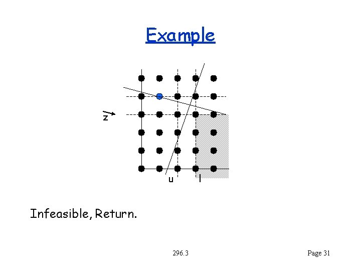
Example z u l Infeasible, Return. 296. 3 Page 31

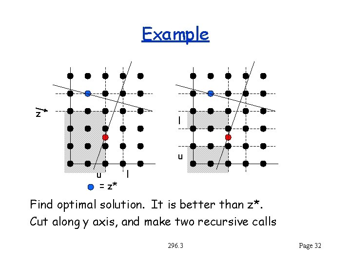
Example z l u u l = z* Find optimal solution. It is better than z*. Cut along y axis, and make two recursive calls 296. 3 Page 32

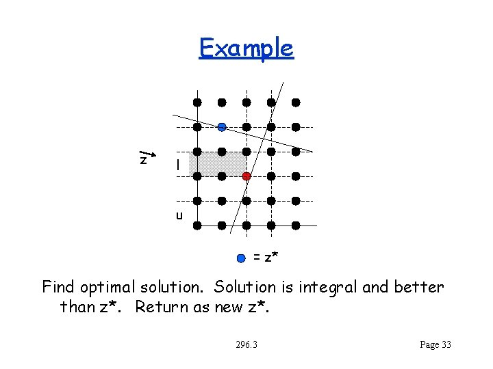
Example z l u = z* Find optimal solution. Solution is integral and better than z*. Return as new z*. 296. 3 Page 33

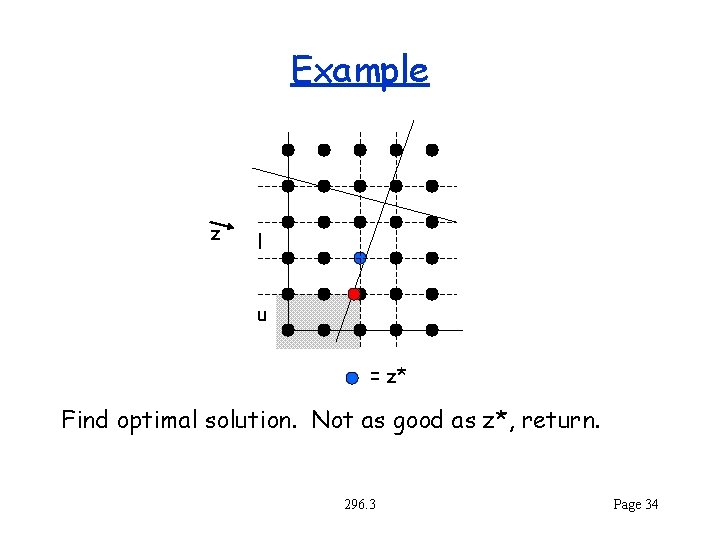
Example z l u = z* Find optimal solution. Not as good as z*, return. 296. 3 Page 34

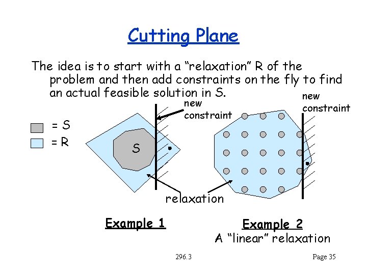
Cutting Plane The idea is to start with a “relaxation” R of the problem and then add constraints on the fly to find an actual feasible solution in S. new =S =R new constraint S relaxation Example 1 Example 2 A “linear” relaxation 296. 3 Page 35

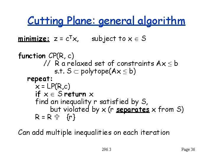
Cutting Plane: general algorithm minimize: z = c. Tx, subject to x S function CP(R, c) // R a relaxed set of constraints Ax ≤ b s. t. S polytope(Ax ≤ b) repeat: x = LP(R, c) if x S return x find an inequality r satisfied by S, but violated by x (r separates x from S) R = R U {r} Can add multiple inequalities on each iteration 296. 3 Page 36

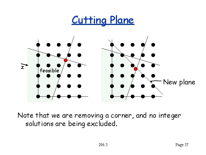
Cutting Plane z feasible New plane Note that we are removing a corner, and no integer solutions are being excluded. 296. 3 Page 37

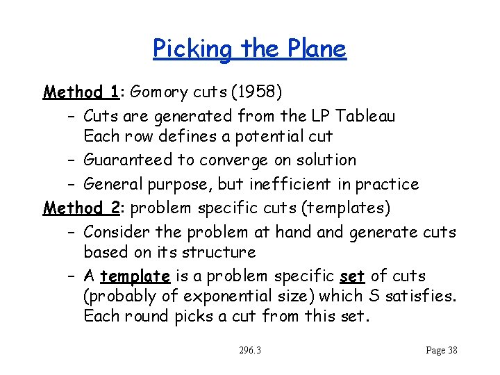
Picking the Plane Method 1: Gomory cuts (1958) – Cuts are generated from the LP Tableau Each row defines a potential cut – Guaranteed to converge on solution – General purpose, but inefficient in practice Method 2: problem specific cuts (templates) – Consider the problem at hand generate cuts based on its structure – A template is a problem specific set of cuts (probably of exponential size) which S satisfies. Each round picks a cut from this set. 296. 3 Page 38

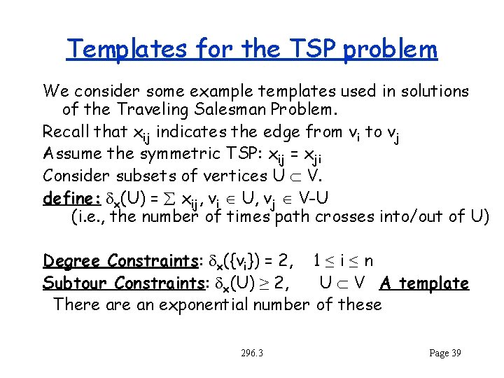
Templates for the TSP problem We consider some example templates used in solutions of the Traveling Salesman Problem. Recall that xij indicates the edge from vi to vj Assume the symmetric TSP: xij = xji Consider subsets of vertices U V. define: dx(U) = å xij, vi U, vj V-U (i. e. , the number of times path crosses into/out of U) Degree Constraints: dx({vi}) = 2, 1 ≤ i ≤ n Subtour Constraints: dx(U) ≥ 2, U V A template There an exponential number of these 296. 3 Page 39

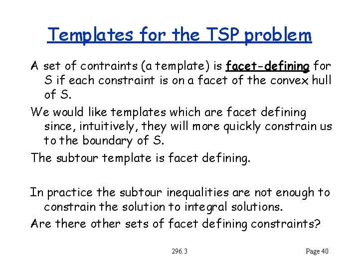
Templates for the TSP problem A set of contraints (a template) is facet-defining for S if each constraint is on a facet of the convex hull of S. We would like templates which are facet defining since, intuitively, they will more quickly constrain us to the boundary of S. The subtour template is facet defining. In practice the subtour inequalities are not enough to constrain the solution to integral solutions. Are there other sets of facet defining constraints? 296. 3 Page 40

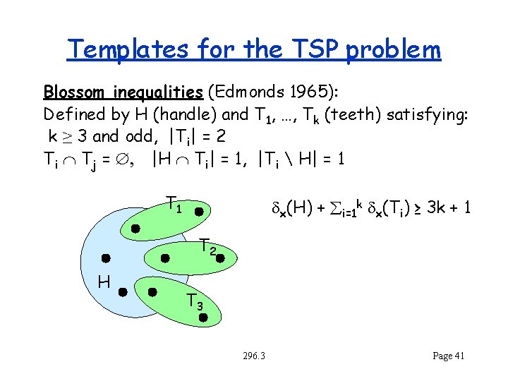
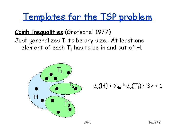
Templates for the TSP problem Blossom inequalities (Edmonds 1965): Defined by H (handle) and T 1, …, Tk (teeth) satisfying: k ≥ 3 and odd, |Ti| = 2 Ti Tj = Æ, |H Ti| = 1, |Ti H| = 1 T 1 dx(H) + åi=1 k dx(Ti) ≥ 3 k + 1 T 2 H T 3 296. 3 Page 41

Templates for the TSP problem Comb inequalities (Grotschel 1977) Just generalizes Ti to be any size. At least one element of each Ti has to be in and out of H. T 1 T 2 H dx(H) + åi=1 k dx(Ti) ≥ 3 k + 1 T 3 296. 3 Page 42

The art of Templates Picking the right set of templates, and applying them in the right way is the art of solving NP-hard problems with integer programming. Different problems have different templates. One needs to find good algorithms for selecting a member of a template that separates x from S (can be quite complicated on its own). Cutting planes often used in conjunction with branch and bound. Can interleave template cuts with Gomory cuts (e. g. , use Gomory cuts when the set of template cuts “dries out”). 296. 3 Page 43

Practical Developments • Good formulations, heuristics and theory Goal: to get LP solution as close as possible to IP solution Disaggregation, adding constraints (cuts) • Preprocessing Automatic methods for reformulation Some interesting graph theory is involved • Cut generation (branch-and-cut) Add cuts during the branch-and-bound • Column generation Improve formulation by introducing an exponential number of variables. 296. 3 Page 44