CPS 296 3 Algorithms in the Real World

CPS 296. 3: Algorithms in the Real World Data Compression: Lecture 2. 5 296. 3 1

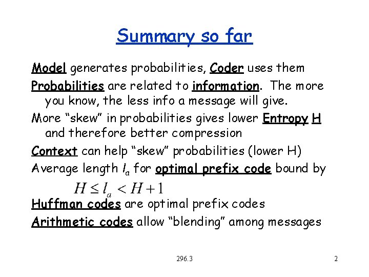
Summary so far Model generates probabilities, Coder uses them Probabilities are related to information. The more you know, the less info a message will give. More “skew” in probabilities gives lower Entropy H and therefore better compression Context can help “skew” probabilities (lower H) Average length la for optimal prefix code bound by Huffman codes are optimal prefix codes Arithmetic codes allow “blending” among messages 296. 3 2

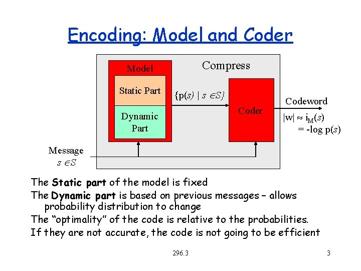
Encoding: Model and Coder Compress Model Static Part {p(s) | s S} Coder Dynamic Part Codeword |w| i. M(s) = -log p(s) Message s S The Static part of the model is fixed The Dynamic part is based on previous messages – allows probability distribution to change The “optimality” of the code is relative to the probabilities. If they are not accurate, the code is not going to be efficient 296. 3 3

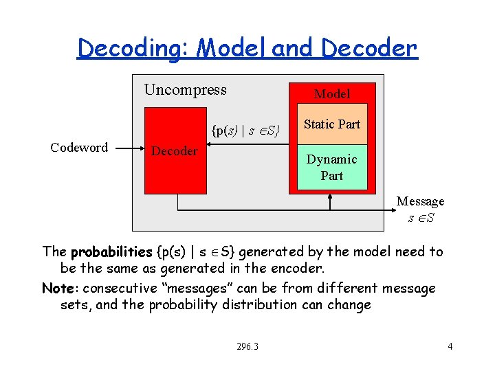
Decoding: Model and Decoder Uncompress Model {p(s) | s S} Codeword Decoder Static Part Dynamic Part Message s S The probabilities {p(s) | s S} generated by the model need to be the same as generated in the encoder. Note: consecutive “messages” can be from different message sets, and the probability distribution can change 296. 3 4

Codes with Dynamic Probabilities Huffman codes: Need to generate a new tree for new probabilities. Small changes in probability typically make small changes to the Huffman tree. “Adaptive Huffman codes” update the tree without having to completely recalculate it. Used frequently in practice Arithmetic codes: Need to recalculate the f(m) values based on current probabilities. Can be done with a balanced tree. 296. 3 5

Compression Outline Introduction: Lossy vs. Lossless, Benchmarks, … Information Theory: Entropy, etc. Probability Coding: Huffman + Arithmetic Coding Applications of Probability Coding: PPM + others – Transform coding: move to front, run-length, … – Context coding: fixed context, partial matching Lempel-Ziv Algorithms: LZ 77, gzip, compress, . . . Other Lossless Algorithms: Burrows-Wheeler Lossy algorithms for images: JPEG, MPEG, . . . Compressing graphs and meshes: BBK 296. 3 6

Applications of Probability Coding How do we generate the probabilities? Using character frequencies directly does not work very well (e. g. 4. 5 bits/char for text). Technique 1: transforming the data – Run length coding (ITU Fax standard) – Move-to-front coding (Used in Burrows-Wheeler) – Residual coding (JPEG LS) Technique 2: using conditional probabilities – Fixed context (JBIG…almost) – Partial pattern matching (PPM) 296. 3 7

Run Length Coding Code by specifying message value followed by the number of repeated values: e. g. abbbaacccca => (a, 1), (b, 3), (a, 2), (c, 4), (a, 1) The characters and counts can be coded based on frequency, ensures only a few bits of overhead for low counts such as 1. Run length coding exploits context to skew probabilities. 296. 3 8

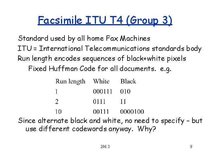
Facsimile ITU T 4 (Group 3) Standard used by all home Fax Machines ITU = International Telecommunications standards body Run length encodes sequences of black+white pixels Fixed Huffman Code for all documents. e. g. Since alternate black and white, no need to specify – but use different codewords anyway. Why? 296. 3 9

Facsimile ITU T 4 (Group 3) Transform: (run length) – input : binary string – output : interleaving of run lengths of black and white pixels Probabilities: (on the output of the transform) Static probabilities of each run length based on large set of test documents. Coding: Huffman coding 296. 3 10

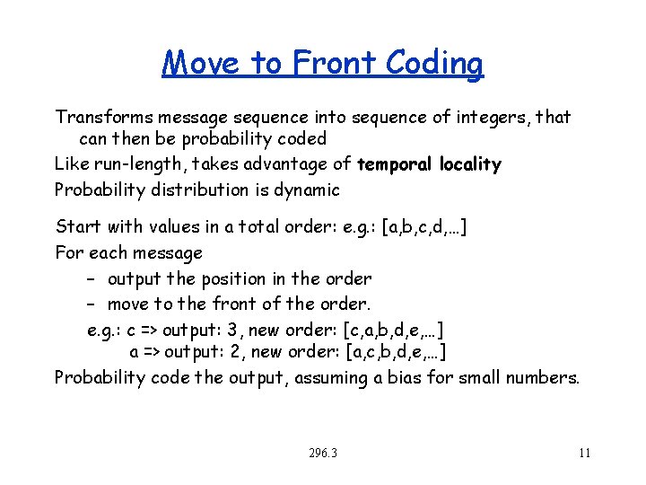
Move to Front Coding Transforms message sequence into sequence of integers, that can then be probability coded Like run-length, takes advantage of temporal locality Probability distribution is dynamic Start with values in a total order: e. g. : [a, b, c, d, …] For each message – output the position in the order – move to the front of the order. e. g. : c => output: 3, new order: [c, a, b, d, e, …] a => output: 2, new order: [a, c, b, d, e, …] Probability code the output, assuming a bias for small numbers. 296. 3 11

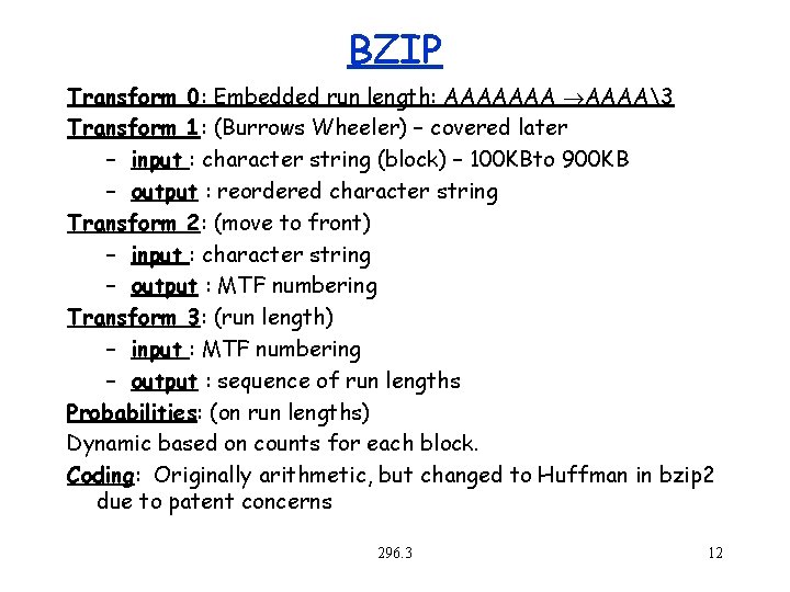
BZIP Transform 0: Embedded run length: AAAAAAA3 Transform 1: (Burrows Wheeler) – covered later – input : character string (block) – 100 KBto 900 KB – output : reordered character string Transform 2: (move to front) – input : character string – output : MTF numbering Transform 3: (run length) – input : MTF numbering – output : sequence of run lengths Probabilities: (on run lengths) Dynamic based on counts for each block. Coding: Originally arithmetic, but changed to Huffman in bzip 2 due to patent concerns 296. 3 12

Residual Coding Typically used for message values that represent some sort of amplitude: e. g. , gray-level in an image, or amplitude in audio. Basic Idea: guess next value based on current context. Output difference between guess and actual value. Use probability code on the output. Consider compressing a stock value over time. 296. 3 13

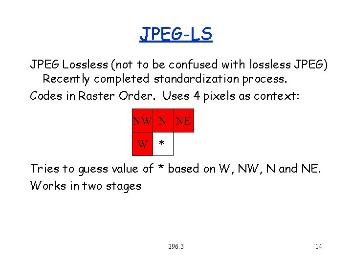
JPEG-LS JPEG Lossless (not to be confused with lossless JPEG) Recently completed standardization process. Codes in Raster Order. Uses 4 pixels as context: NW N NE W * Tries to guess value of * based on W, N and NE. Works in two stages 296. 3 14

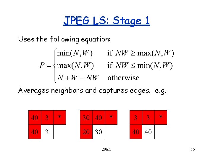
JPEG LS: Stage 1 Uses the following equation: Averages neighbors and captures edges. e. g. 40 3 * 30 40 * 3 20 30 40 40 296. 3 3 * 15

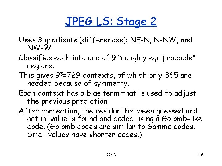
JPEG LS: Stage 2 Uses 3 gradients (differences): NE-N, N-NW, and NW-W Classifies each into one of 9 “roughly equiprobable” regions. This gives 93=729 contexts, of which only 365 are needed because of symmetry. Each context has a bias term that is used to adjust the previous prediction After correction, the residual between guessed and actual value is found and coded using a Golomb-like code. (Golomb codes are similar to Gamma codes. Small values have shorter codes. ) 296. 3 16

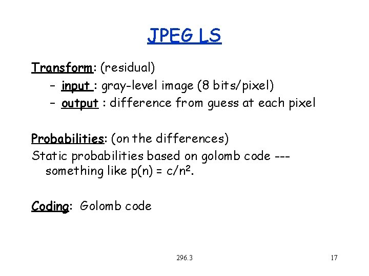
JPEG LS Transform: (residual) – input : gray-level image (8 bits/pixel) – output : difference from guess at each pixel Probabilities: (on the differences) Static probabilities based on golomb code --something like p(n) = c/n 2. Coding: Golomb code 296. 3 17

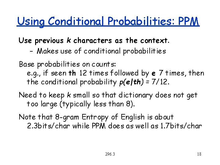
Using Conditional Probabilities: PPM Use previous k characters as the context. – Makes use of conditional probabilities Base probabilities on counts: e. g. , if seen th 12 times followed by e 7 times, then the conditional probability p(e|th) = 7/12. Need to keep k small so that dictionary does not get too large (typically less than 8). Note that 8 -gram Entropy of English is about 2. 3 bits/char while PPM does as well as 1. 7 bits/char 296. 3 18

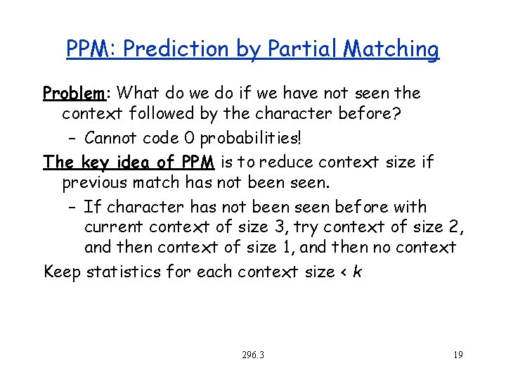
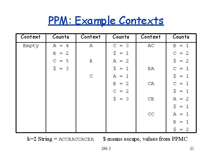
PPM: Prediction by Partial Matching Problem: What do we do if we have not seen the context followed by the character before? – Cannot code 0 probabilities! The key idea of PPM is to reduce context size if previous match has not been seen. – If character has not been seen before with current context of size 3, try context of size 2, and then context of size 1, and then no context Keep statistics for each context size < k 296. 3 19

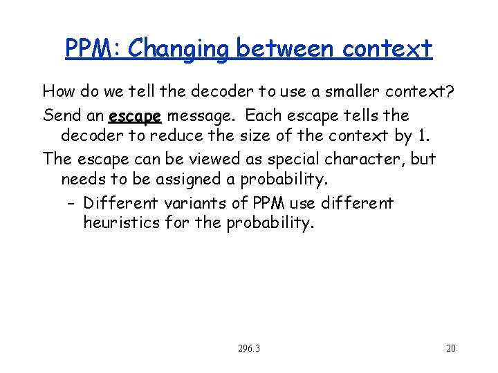
PPM: Changing between context How do we tell the decoder to use a smaller context? Send an escape message. Each escape tells the decoder to reduce the size of the context by 1. The escape can be viewed as special character, but needs to be assigned a probability. – Different variants of PPM use different heuristics for the probability. 296. 3 20

PPM: Example Contexts Context Empty Counts A B C $ = = 4 2 5 3 Context Counts A C $ A B C $ B C = = = = 3 1 2 1 1 2 2 3 Context AC BA CA CB CC k=2 String = ACCBACCACBA Counts B C $ C $ A B $ = = = 1 2 2 1 1 1 2 $ means escape, values from PPMC 296. 3 21

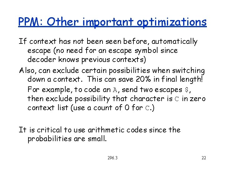
PPM: Other important optimizations If context has not been seen before, automatically escape (no need for an escape symbol since decoder knows previous contexts) Also, can exclude certain possibilities when switching down a context. This can save 20% in final length! For example, to code an A, send two escapes $, then exclude possibility that character is C in zero context list (use a count of 0 for C. ) It is critical to use arithmetic codes since the probabilities are small. 296. 3 22