0 VS 452 5 EN 253 Lecture 8

0 VS 452 + 5 EN 253 Lecture 8 (part II) + Lecture 9 IS-LM MODEL AND AD-AS MODEL Eva Hromádková, 12. 4 2010 + 19. 4 2010

Overview of Lecture 8 – part II 2 IS-LM model of AD curve: Model for AD curve => analysis of stabilization policies IS curve – goods market LM curve – money market Fiscal policy – expenditures and taxes Monetary policy – money supply Equilibrium – interest rates (slides by Ron Cronowich)

IS-LM model Context 3 q We have already introduced the model of aggregate demand (QTM) and aggregate supply. q Long run § prices flexible § output determined by factors of production & technology § unemployment equals its natural rate q. Short run § prices fixed § output determined by aggregate demand § unemployment is negatively related to output

IS-LM model Context II 4 q Today we will develop IS-LM model, theory that explains the aggregate demand curve q First, we focus on the short run and assume hat price level is fixed q Then, we allow price to be flexible, and derive AD curve q Finally, we analyze the effect of fiscal and monetary policy on the most important macroeconomic aggregates – output and unemployment

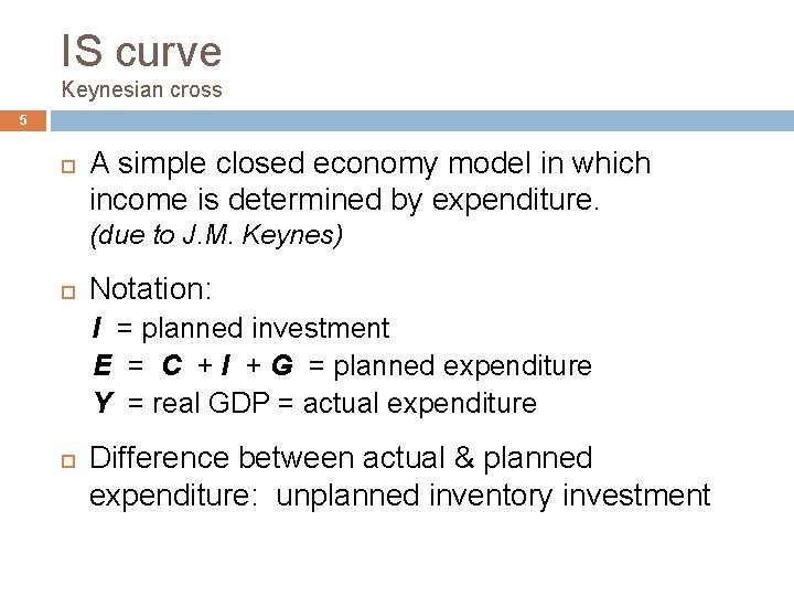
IS curve Keynesian cross 5 A simple closed economy model in which income is determined by expenditure. (due to J. M. Keynes) Notation: I = planned investment E = C + I + G = planned expenditure Y = real GDP = actual expenditure Difference between actual & planned expenditure: unplanned inventory investment

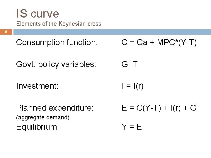
IS curve Elements of the Keynesian cross 6 Consumption function: C = Ca + MPC*(Y-T) Govt. policy variables: G, T Investment: I = I(r) Planned expenditure: E = C(Y-T) + I(r) + G (aggregate demand) Equilibrium: Y=E

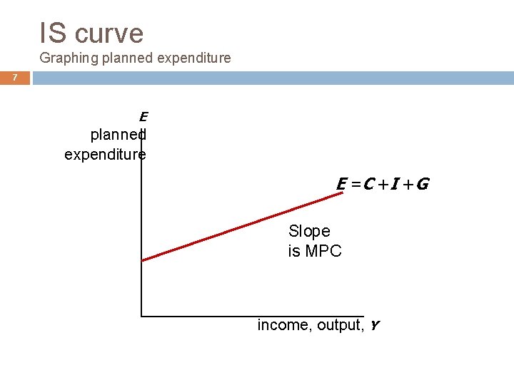
IS curve Graphing planned expenditure 7 E planned expenditure E = C +I +G Slope is MPC income, output, Y

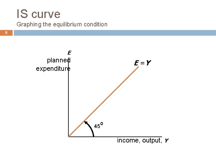
IS curve Graphing the equilibrium condition 8 E planned expenditure E =Y 45º income, output, Y

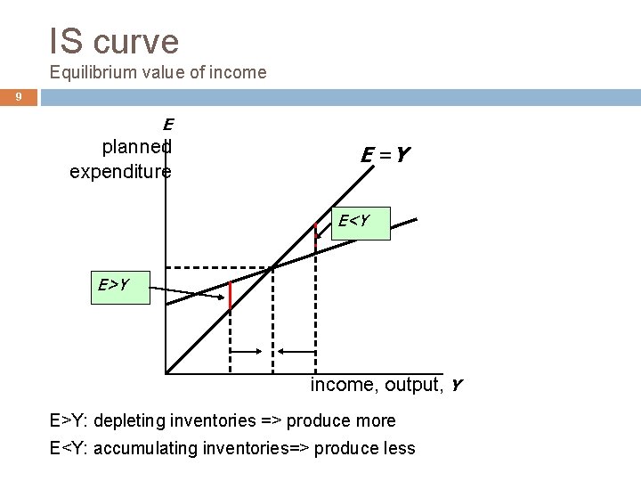
IS curve Equilibrium value of income 9 E planned expenditure E =Y E<Y E>Y income, output, Y E>Y: depleting inventories => produce more E<Y: accumulating inventories=> produce less

IS curve Fiscal policy 10 Fiscal stimulus: Increase in government expenditures Cut taxes Increase transfer payments Fiscal restraint: Decrease in government expenditures Increased taxes Decreased transfer payments

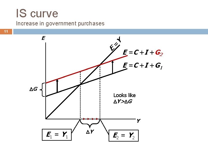
IS curve Increase in government purchases 11 = E E Y E = C + I + G 2 E = C + I + G 1 G Looks like Y> G Y E 1 = Y 1 Y E 2 = Y 2

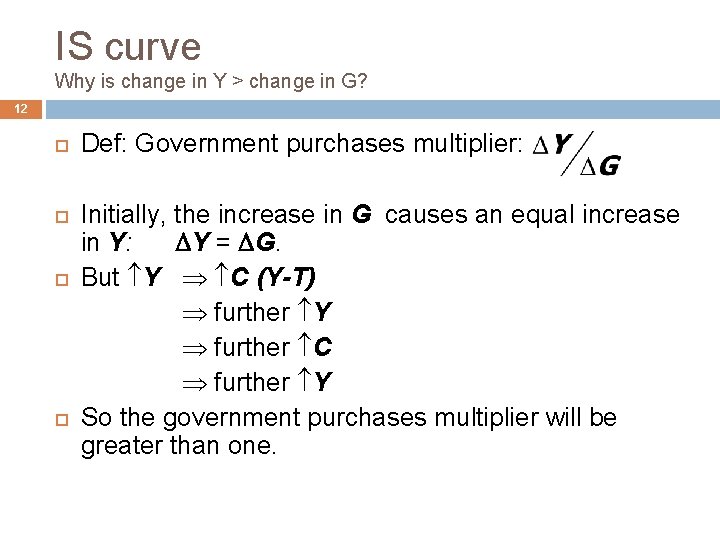
IS curve Why is change in Y > change in G? 12 Def: Government purchases multiplier: Initially, the increase in G causes an equal increase in Y: Y = G. But Y C (Y-T) further Y further C further Y So the government purchases multiplier will be greater than one.

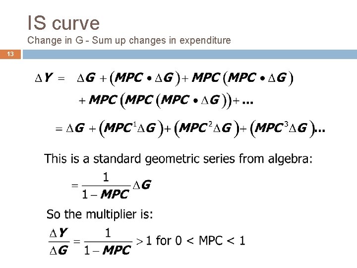
IS curve Change in G - Sum up changes in expenditure 13

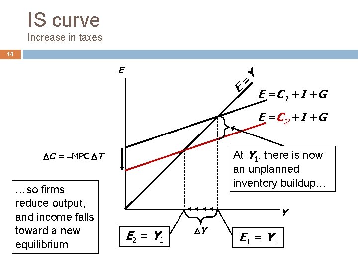
IS curve Increase in taxes 14 = E E Y E = C 1 +I +G E = C 2 +I +G At Y 1, there is now an unplanned inventory buildup… C = MPC T …so firms reduce output, and income falls toward a new equilibrium Y E 2 = Y 2 Y E 1 = Y 1

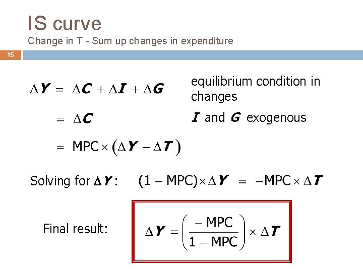
IS curve Change in T - Sum up changes in expenditure 15 equilibrium condition in changes I and G exogenous Solving for Y : Final result:

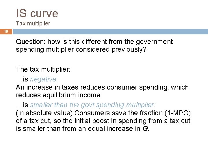
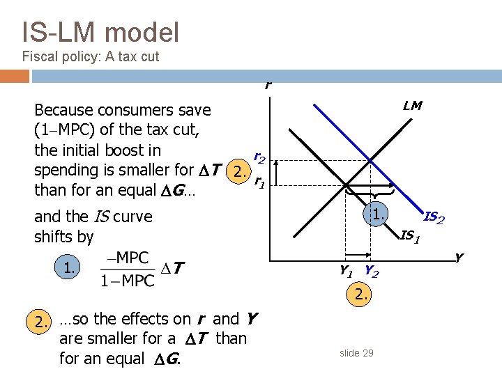
IS curve Tax multiplier 16 Question: how is this different from the government spending multiplier considered previously? The tax multiplier: …is negative: An increase in taxes reduces consumer spending, which reduces equilibrium income. …is smaller than the govt spending multiplier: (in absolute value) Consumers save the fraction (1 -MPC) of a tax cut, so the initial boost in spending from a tax cut is smaller than from an equal increase in G.

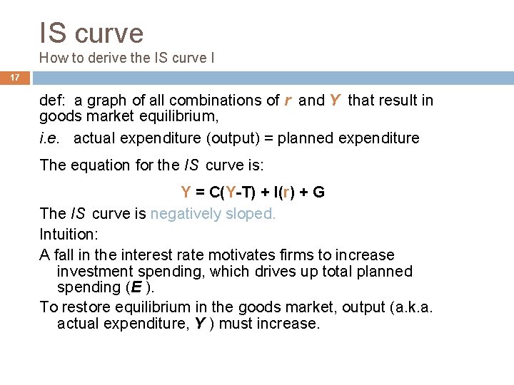
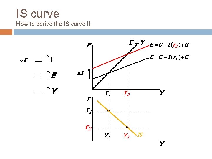
IS curve How to derive the IS curve I 17 def: a graph of all combinations of r and Y that result in goods market equilibrium, i. e. actual expenditure (output) = planned expenditure The equation for the IS curve is: Y = C(Y-T) + I(r) + G The IS curve is negatively sloped. Intuition: A fall in the interest rate motivates firms to increase investment spending, which drives up total planned spending (E ). To restore equilibrium in the goods market, output (a. k. a. actual expenditure, Y ) must increase.

IS curve How to derive the IS curve II E =Y E E =C +I (r 1 )+G r I E Y E =C +I (r 2 )+G I r Y 1 Y 2 Y r 1 r 2 IS Y

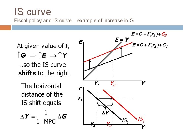
IS curve Fiscal policy and IS curve – example of increase in G At given value of r, G E Y E =Y E E =C +I (r 1 )+G 2 E =C +I (r 1 )+G 1 …so the IS curve shifts to the right. The horizontal distance of the IS shift equals r Y 1 Y Y 2 r 1 Y Y 1 Y 2 IS 1 IS 2 Y

LM curve How to build the LM curve 20 The theory of liquidity preference: Developed by John Maynard Keynes. A simple theory in which the interest rate is determined by money supply and money demand.

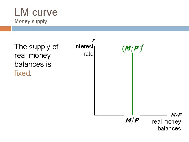
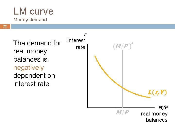
LM curve Money supply The supply of real money balances is fixed. r interest rate M/P real money balances

LM curve Money demand 22 r The demand for real money balances is negatively dependent on interest rate L (r, Y ) M/P real money balances

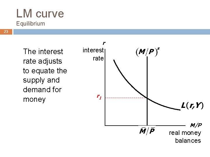
LM curve Equilibrium 23 r The interest rate adjusts to equate the supply and demand for money interest rate r 1 L (r, Y ) M/P real money balances

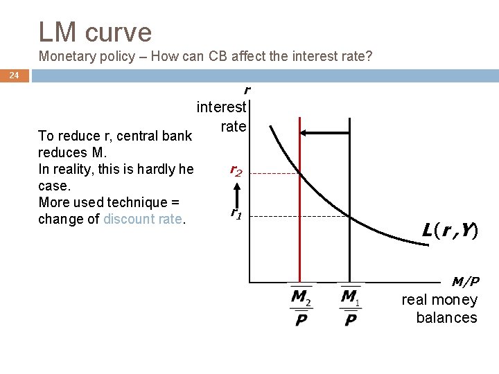
LM curve Monetary policy – How can CB affect the interest rate? 24 r To reduce r, central bank reduces M. In reality, this is hardly he case. More used technique = change of discount rate. interest rate r 2 r 1 L (r , Y) M/P real money balances

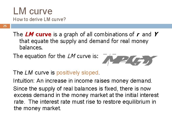
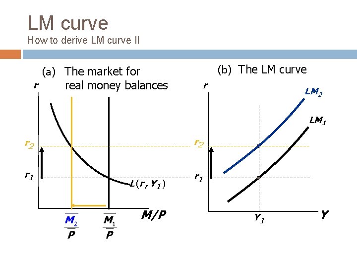
LM curve How to derive LM curve? 25 The LM curve is a graph of all combinations of r and Y that equate the supply and demand for real money balances. The equation for the LM curve is: The LM curve is positively sloped. Intuition: An increase in income raises money demand. Since the supply of real balances is fixed, there is now excess demand in the money market at the initial interest rate. The interest rate must rise to restore equilibrium in the money market.

LM curve How to derive LM curve II (b) The LM curve (a) The market for r real money balances r LM 2 LM 1 r 2 r 1 L ( r , Y 1 ) M/P r 1 Y

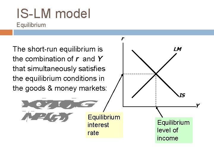
IS-LM model Equilibrium r The short-run equilibrium is the combination of r and Y that simultaneously satisfies the equilibrium conditions in the goods & money markets: LM IS Y Equilibrium interest rate Equilibrium level of income

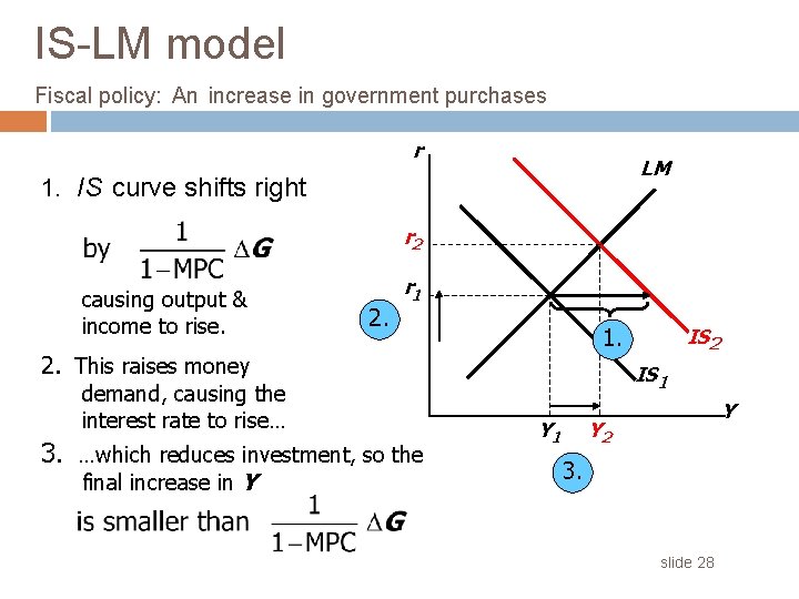
IS-LM model Fiscal policy: An increase in government purchases r LM 1. IS curve shifts right r 2 causing output & income to rise. 2. r 1 2. This raises money demand, causing the interest rate to rise… 3. …which reduces investment, so the final increase in Y IS 2 1. IS 1 Y Y 2 3. slide 28

IS-LM model Fiscal policy: A tax cut r LM Because consumers save (1 MPC) of the tax cut, the initial boost in r 2 spending is smaller for T 2. r 1 than for an equal G… 1. and the IS curve shifts by 1. IS 1 Y 2 2. 2. …so the effects on r and Y are smaller for a T than for an equal G. IS 2 slide 29 Y

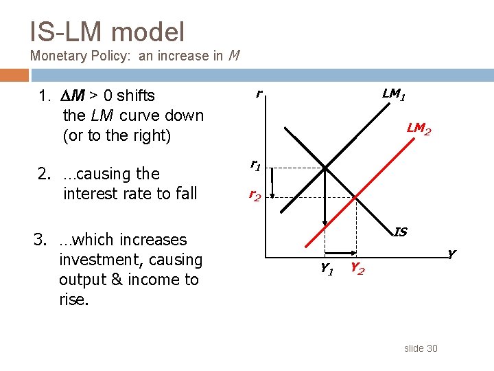
IS-LM model Monetary Policy: an increase in M 1. M > 0 shifts the LM curve down (or to the right) 2. …causing the interest rate to fall 3. …which increases investment, causing output & income to rise. r LM 1 LM 2 r 1 r 2 IS Y 1 Y Y 2 slide 30

IS-LM model Shocks I 31 LM shocks: exogenous changes in the demand for money. Examples: • • a wave of credit card fraud increases demand for money more ATMs or the Internet banking reduce money demand

IS-LM model Shocks II 32 IS shocks: exogenous changes in the demand for goods & services. Examples: • • stock market boom or crash change in households’ wealth C change in business or consumer confidence or expectations I and/or C

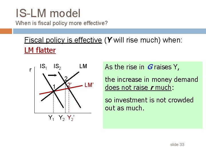
IS-LM model When is fiscal policy more effective? Fiscal policy is effective (Y will rise much) when: LM flatter r IS 1 IS 2 1 LM 2 2’ LM’ As the rise in G raises Y, the increase in money demand does not raise r much: so investment is not crowded out as much. Y 1 Y 2 ’ slide 33

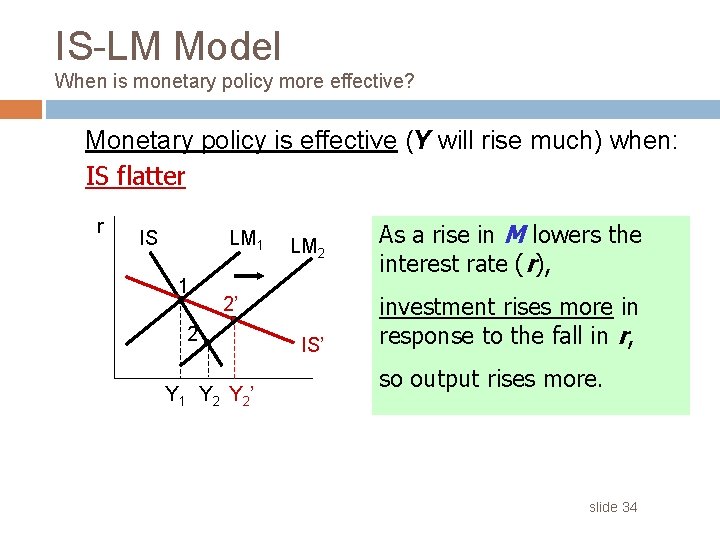
IS-LM Model When is monetary policy more effective? Monetary policy is effective (Y will rise much) when: IS flatter r IS LM 1 1 LM 2 2’ 2 Y 1 Y 2 ’ IS’ As a rise in M lowers the interest rate (r), investment rises more in response to the fall in r, so output rises more. slide 34

Aggregate demand How to get from IS-LM to AD 35 So far, we’ve been using the IS-LM model to analyze the short run, when the price level is assumed fixed. However, a change in P would shift the LM curve and therefore affect Y. The aggregate demand curve (introduced in chap. 9 ) captures this relationship between P and Y

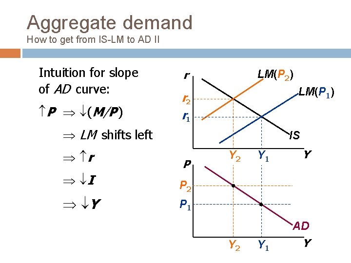
Aggregate demand How to get from IS-LM to AD II Intuition for slope of AD curve: P (M/P ) r LM(P 2) LM(P 1) r 2 r 1 LM shifts left r I Y IS P Y 2 Y 1 Y P 2 P 1 AD Y 2 Y 1 Y

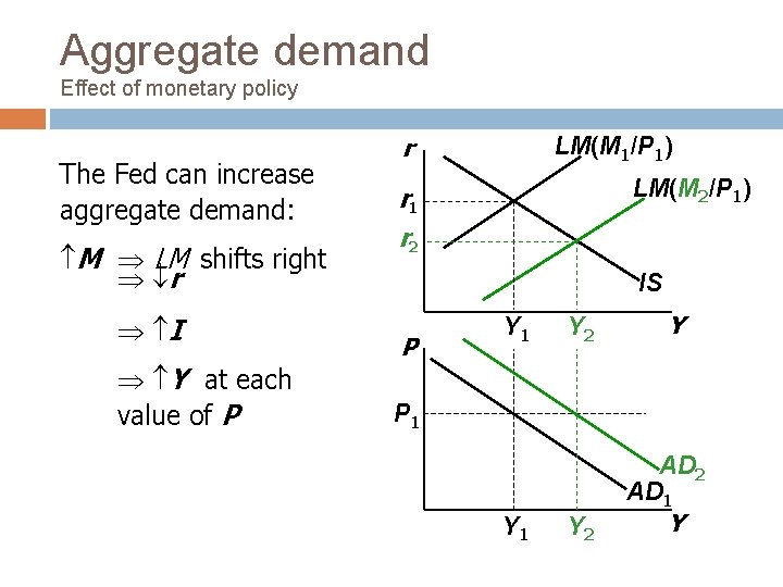
Aggregate demand Effect of monetary policy The Fed can increase aggregate demand: M LM shifts right r I Y at each value of P r LM(M 1/P 1) LM(M 2/P 1) r 1 r 2 IS P Y 1 Y 2 Y P 1 Y 2 AD 1 Y

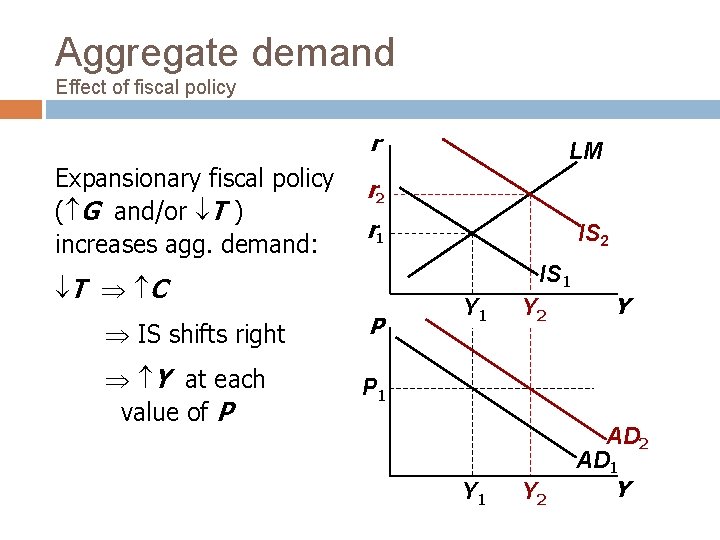
Aggregate demand Effect of fiscal policy r Expansionary fiscal policy ( G and/or T ) increases agg. demand: LM r 2 r 1 IS 2 IS 1 T C IS shifts right P Y at each value of P P 1 Y 1 Y 2 Y AD 2 AD 1 Y

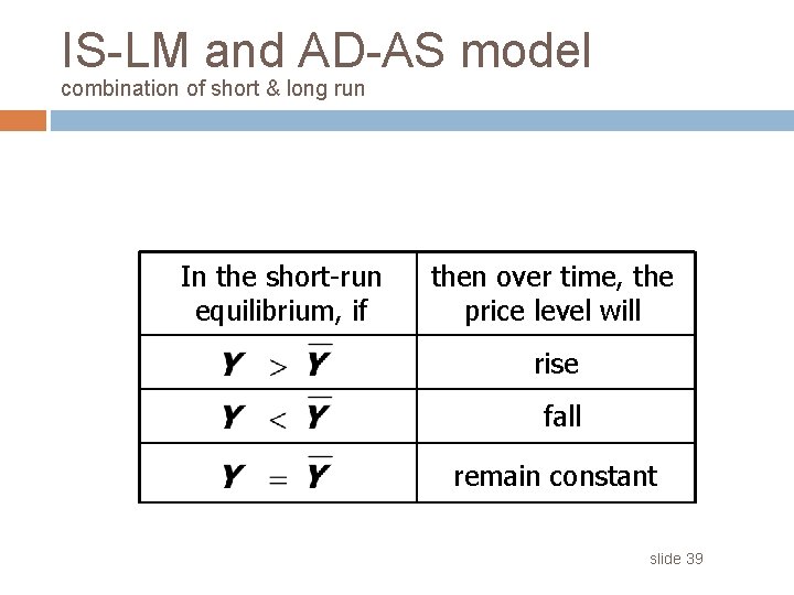
IS-LM and AD-AS model combination of short & long run In the short-run equilibrium, if then over time, the price level will rise fall remain constant slide 39

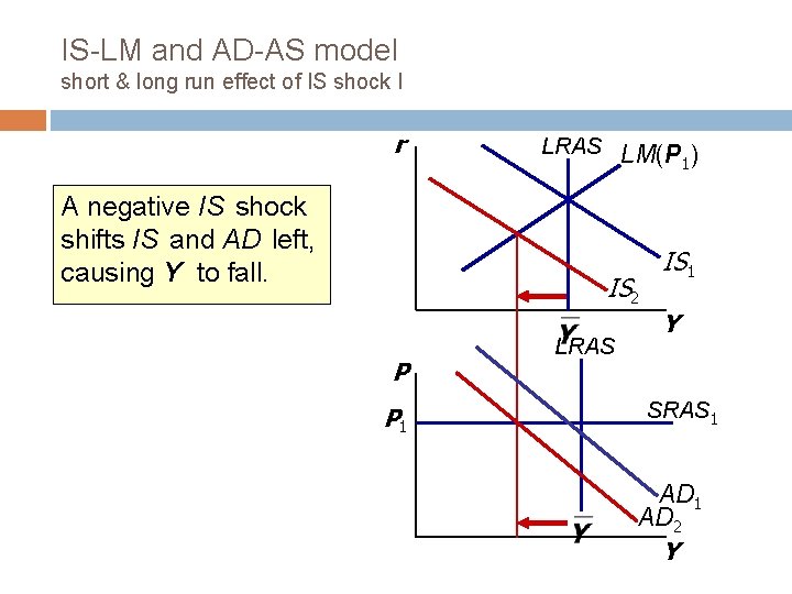
IS-LM and AD-AS model short & long run effect of IS shock I r A negative IS shock shifts IS and AD left, causing Y to fall. LRAS LM(P ) 1 IS 2 P P 1 LRAS IS 1 Y SRAS 1 AD 2 Y

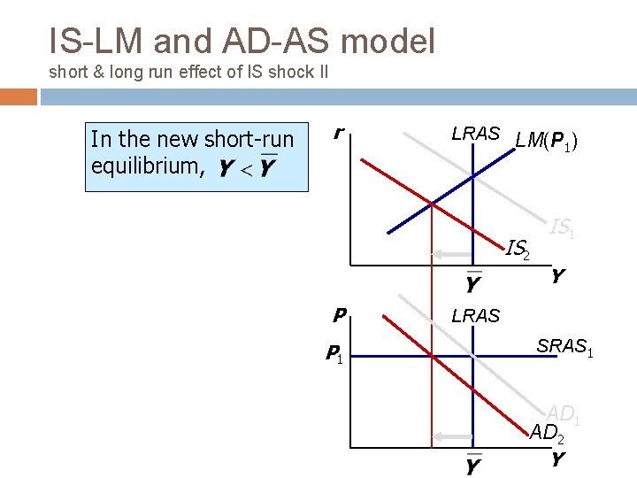
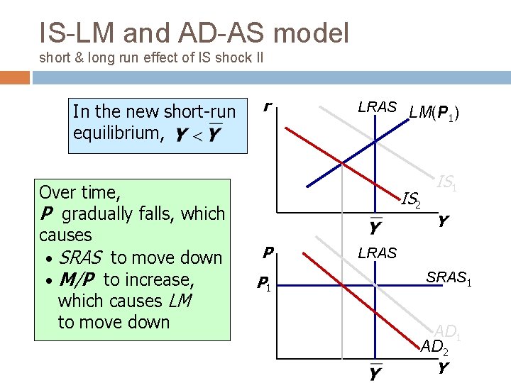
IS-LM and AD-AS model short & long run effect of IS shock II In the new short-run equilibrium, r LRAS LM(P ) 1 IS 2 IS 1 Y P P 1 LRAS SRAS 1 AD 2 Y

IS-LM and AD-AS model short & long run effect of IS shock II In the new short-run equilibrium, Over time, P gradually falls, which causes • SRAS to move down • M/P to increase, which causes LM to move down r LRAS LM(P ) 1 IS 2 IS 1 Y P P 1 LRAS SRAS 1 AD 2 Y

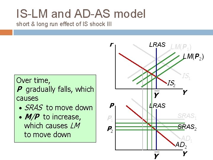
IS-LM and AD-AS model short & long run effect of IS shock III r LRAS LM(P ) 1 LM(P 2) Over time, P gradually falls, which causes • SRAS to move down • M/P to increase, which causes LM to move down IS 2 IS 1 Y P LRAS P 1 SRAS 1 P 2 SRAS 2 AD 1 AD 2 Y

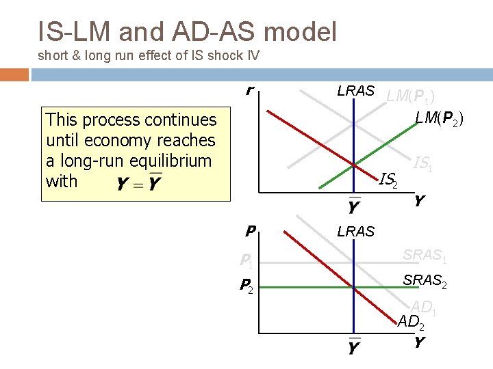
IS-LM and AD-AS model short & long run effect of IS shock IV r LRAS LM(P ) 1 LM(P 2) This process continues until economy reaches a long-run equilibrium with IS 2 IS 1 Y P LRAS P 1 SRAS 1 P 2 SRAS 2 AD 1 AD 2 Y

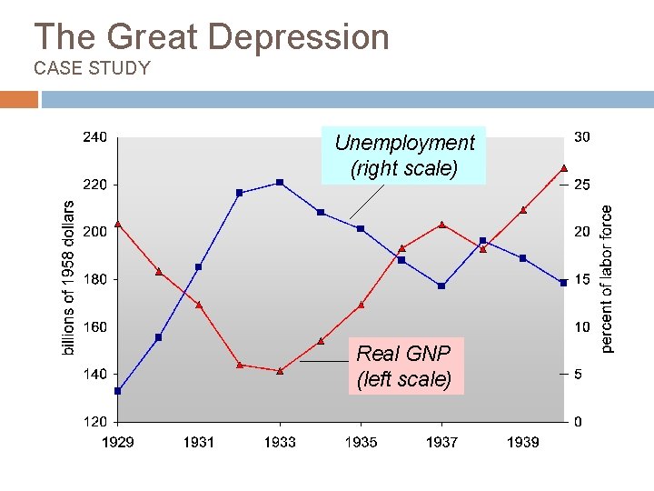
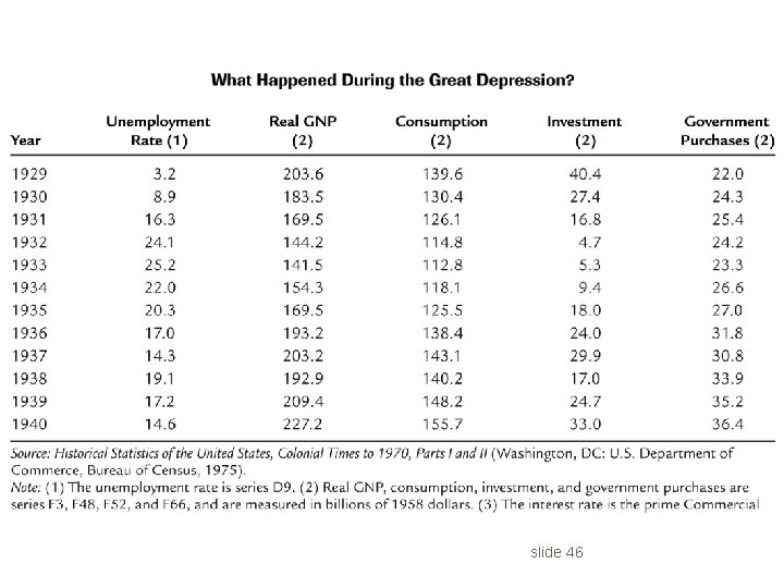
The Great Depression CASE STUDY Unemployment (right scale) Real GNP (left scale)

slide 46

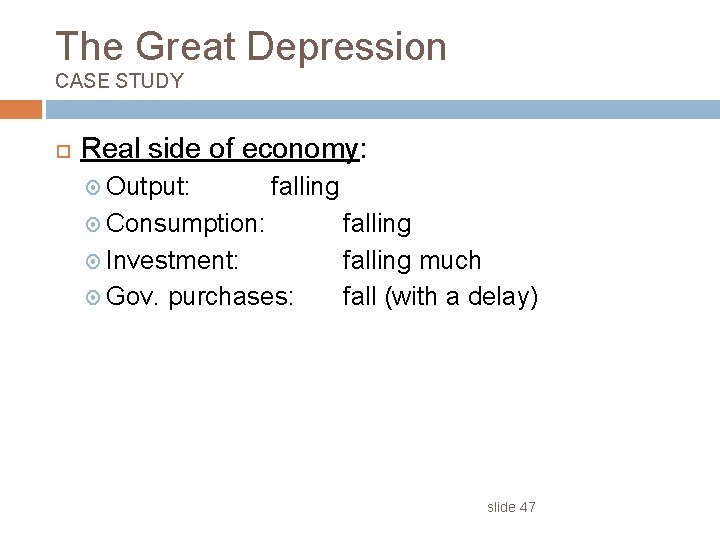
The Great Depression CASE STUDY Real side of economy: Output: falling Consumption: Investment: Gov. purchases: falling much fall (with a delay) slide 47

slide 48

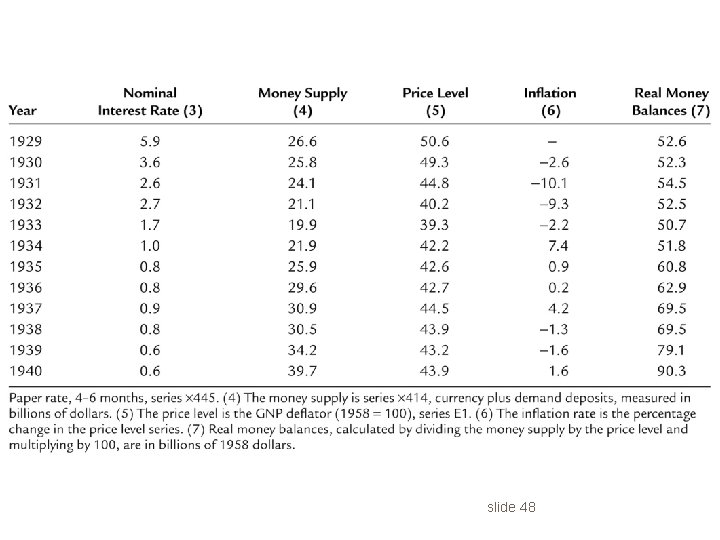
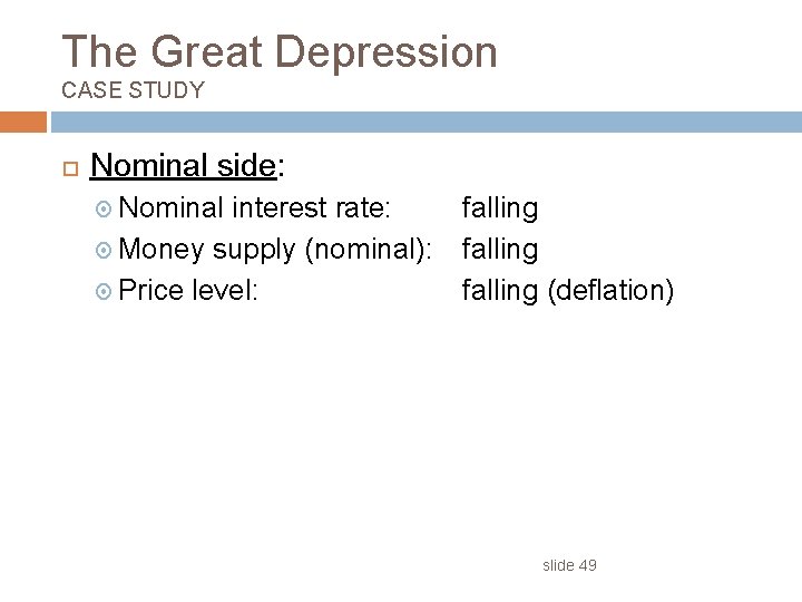
The Great Depression CASE STUDY Nominal side: Nominal interest rate: Money supply (nominal): Price level: falling (deflation) slide 49

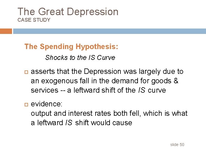
The Great Depression CASE STUDY The Spending Hypothesis: Shocks to the IS Curve asserts that the Depression was largely due to an exogenous fall in the demand for goods & services -- a leftward shift of the IS curve evidence: output and interest rates both fell, which is what a leftward IS shift would cause slide 50

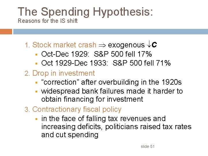
The Spending Hypothesis: Reasons for the IS shift 1. Stock market crash exogenous C Oct-Dec 1929: S&P 500 fell 17% § Oct 1929 -Dec 1933: S&P 500 fell 71% 2. Drop in investment § “correction” after overbuilding in the 1920 s § widespread bank failures made it harder to obtain financing for investment 3. Contractionary fiscal policy § in the face of falling tax revenues and increasing deficits, politicians raised tax rates and cut spending § slide 51

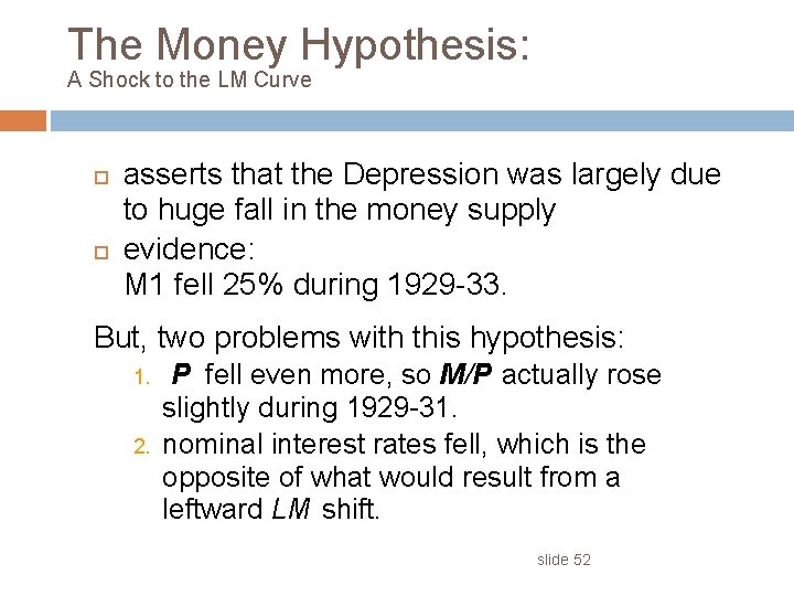
The Money Hypothesis: A Shock to the LM Curve asserts that the Depression was largely due to huge fall in the money supply evidence: M 1 fell 25% during 1929 -33. But, two problems with this hypothesis: 1. 2. P fell even more, so M/P actually rose slightly during 1929 -31. nominal interest rates fell, which is the opposite of what would result from a leftward LM shift. slide 52

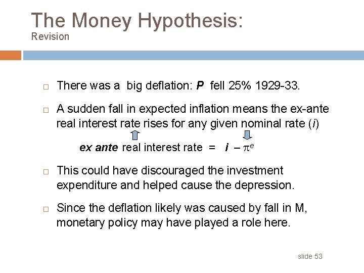
The Money Hypothesis: Revision There was a big deflation: P fell 25% 1929 -33. A sudden fall in expected inflation means the ex-ante real interest rate rises for any given nominal rate (i) ex ante real interest rate = i – e This could have discouraged the investment expenditure and helped cause the depression. Since the deflation likely was caused by fall in M, monetary policy may have played a role here. slide 53