0 VS 452 5 EN 253 Lecture 8

0 VS 452 + 5 EN 253 Lecture 8 – part I BUSINESS CYCLES AND INTRO TO AD-AS MODEL Eva Hromádková, 12. 4 2010

Overview of Lecture 8 – part I 2 Business cycles: Why do we need other than classical model? Puzzle of Great Depression Prices in the short vs. long run Intro to AD and AS curves Effect of shocks in AD-AS model Stabilization policy – tools and goals

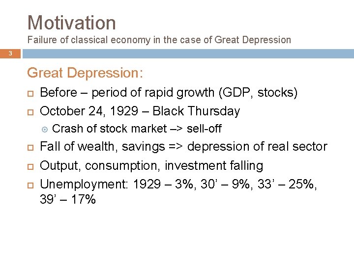
Motivation Failure of classical economy in the case of Great Depression 3 Great Depression: Before – period of rapid growth (GDP, stocks) October 24, 1929 – Black Thursday Crash of stock market –> sell-off Fall of wealth, savings => depression of real sector Output, consumption, investment falling Unemployment: 1929 – 3%, 30’ – 9%, 33’ – 25%, 39’ – 17%

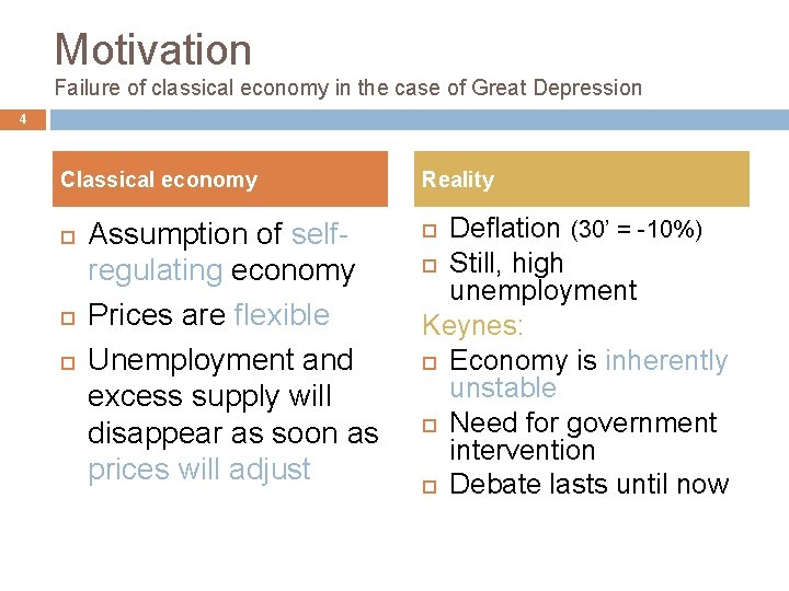
Motivation Failure of classical economy in the case of Great Depression 4 Classical economy Assumption of selfregulating economy Prices are flexible Unemployment and excess supply will disappear as soon as prices will adjust Reality Deflation (30’ = -10%) Still, high unemployment Keynes: Economy is inherently unstable Need for government intervention Debate lasts until now

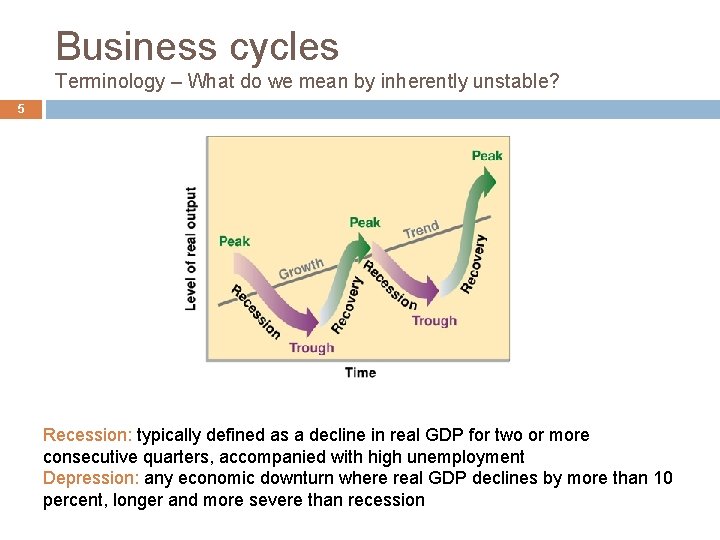
Business cycles Terminology – What do we mean by inherently unstable? 5 Recession: typically defined as a decline in real GDP for two or more consecutive quarters, accompanied with high unemployment Depression: any economic downturn where real GDP declines by more than 10 percent, longer and more severe than recession

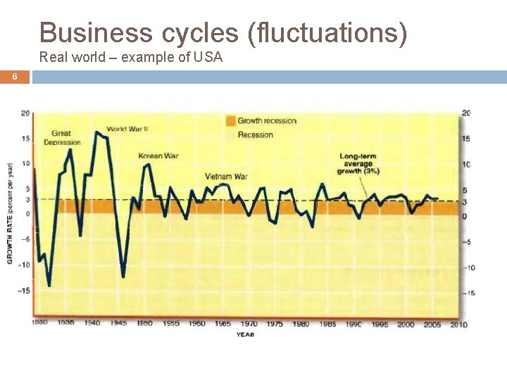
Business cycles (fluctuations) Real world – example of USA 6

Business cycles (fluctuations) Real world – Summary of example of USA 7 Real GDP growth in US: long-run growth of 3. 5% not steady – fluctuations around trend: Great Depression WWII – growth by 19%, all people employed 46’-48’ – postwar depression (military production) 80’s oil crisis

Business cycles (fluctuations) Stylized facts 8 No simple regular or cyclical pattern Distributed unevenly over the components of output Stable: consumption of non-durables and services, net export Unstable: consumption of durables, housing, inventories Asymmetries between rises and falls in output Long time slightly above and short time far below the mean value

Business fluctuations Role of macro theory 9 Macro theory tries to explain why we observe alternating periods of growth and contraction in short run; together with long-term trends Main difference Long-run: prices are flexible, respond to changes in supply or demand Short run: many prices are “sticky” The economy behaves much differently when prices are sticky.

Business fluctuations Comparison of long-term and short-term determinants 10 Long-term (classical economy) Price flexibility Output determined by supply side ( F(K, L) ) Change in demand only affects prices, not quantities Say’s law: supply creates demand Short term (business cycles) Price stickiness Output determined also by demand – affected by exogenous changes Ex: firm – how much we are able to sell at given price

Model of AD and AS 11 the paradigm that most mainstream economists & policymakers use to think about economic fluctuations and policies to stabilize the economy shows how the price level and aggregate output are determined simultaneously shows how the economy’s behavior is different in the short run and long run

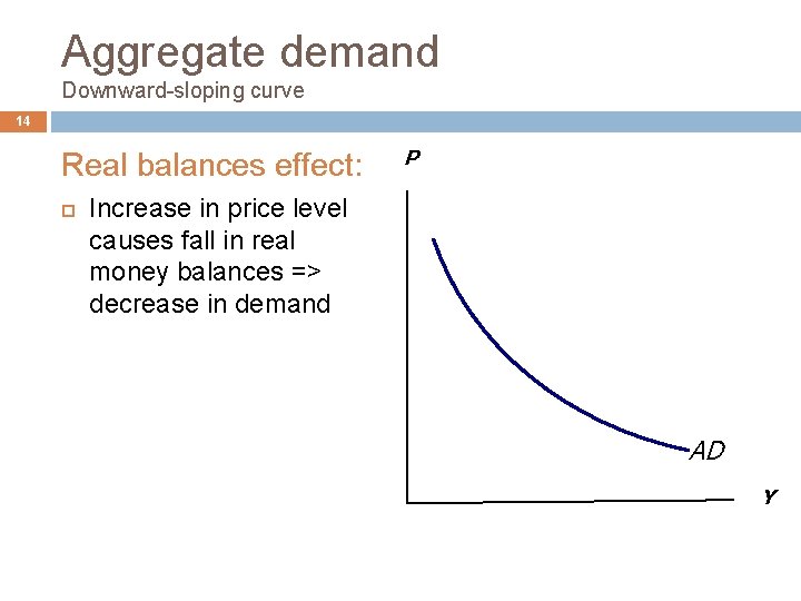
Aggregate demand 12 The aggregate demand curve shows the relationship between the price level and the quantity of output demanded. For this lecture’s intro to the AD/AS model, we use a very simple theory of aggregate demand based on the Quantity Theory of Money. In this and next lecture we develop theory of aggregate demand in more detail.

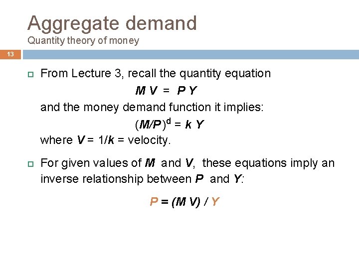
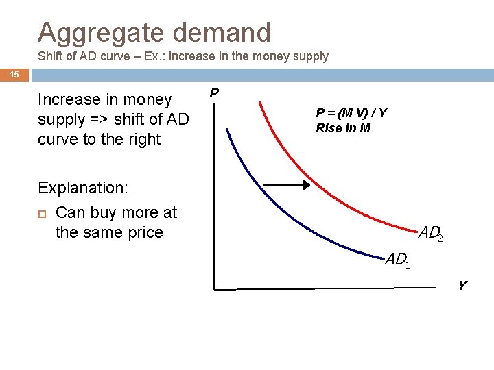
Aggregate demand Quantity theory of money 13 From Lecture 3, recall the quantity equation MV = PY and the money demand function it implies: (M/P )d = k Y where V = 1/k = velocity. For given values of M and V, these equations imply an inverse relationship between P and Y: P = (M V) / Y

Aggregate demand Downward-sloping curve 14 Real balances effect: P Increase in price level causes fall in real money balances => decrease in demand AD Y

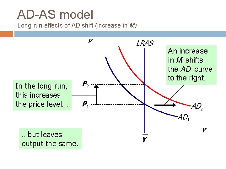
Aggregate demand Shift of AD curve – Ex. : increase in the money supply 15 Increase in money supply => shift of AD curve to the right P P = (M V) / Y Rise in M Explanation: Can buy more at the same price AD 2 AD 1 Y

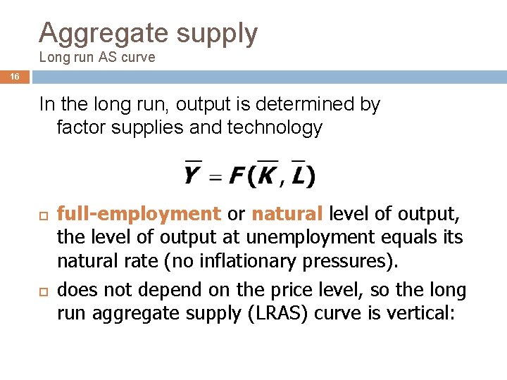
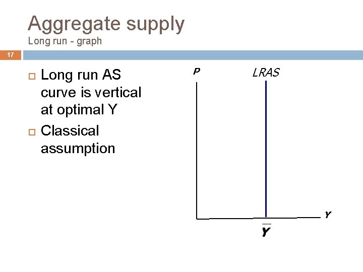
Aggregate supply Long run AS curve 16 In the long run, output is determined by factor supplies and technology full-employment or natural level of output, the level of output at unemployment equals its natural rate (no inflationary pressures). does not depend on the price level, so the long run aggregate supply (LRAS) curve is vertical:

Aggregate supply Long run - graph 17 Long run AS curve is vertical at optimal Y Classical assumption P LRAS Y

AD-AS model Long-run effects of AD shift (increase in M) P In the long run, this increases the price level… P 2 LRAS An increase in M shifts the AD curve to the right. P 1 AD 2 AD 1 …but leaves output the same. Y

AD-AS model Long-run - Implications 19 In the long run – change in the money supply does not have any effect on real variable, only on the price level Deviation only as long as price adjusts Not what we observe in reality! Consider a long term outcome Self-adjusting deviations Economic growth based on the growth of real variables: capital, labor, technology Analyze departures

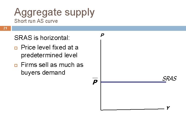
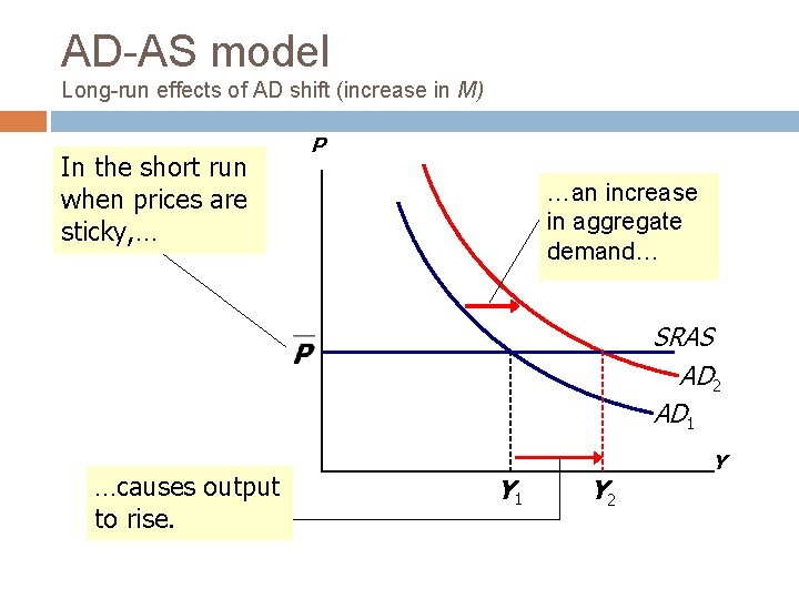
Aggregate supply Short run 20 In the real world, many prices are sticky in the short run. From now on we assume that all prices are stuck at a predetermined level in the short run… …and that firms are willing to sell as much as their customers are willing to buy at that price level. Therefore, the short-run aggregate supply (SRAS) curve is horizontal: (simplification – in reality, upward sloping)

Aggregate supply Short run AS curve 21 SRAS is horizontal: Price level fixed at a predetermined level Firms sell as much as buyers demand P SRAS Y

AD-AS model Long-run effects of AD shift (increase in M) In the short run when prices are sticky, … P …an increase in aggregate demand… SRAS AD 2 AD 1 …causes output to rise. Y 1 Y 2 Y

AD-AS model Short-run - Implications 23 In the short run – change in the AD (money supply) has full effect on real variable + no on price level Equilibrium may be undesirable – higher or lower output (and corresponding prices) than in natural level Lower output – recessionary gap – high unemployment rate Higher output – inflationary gap – pressure to increase prices

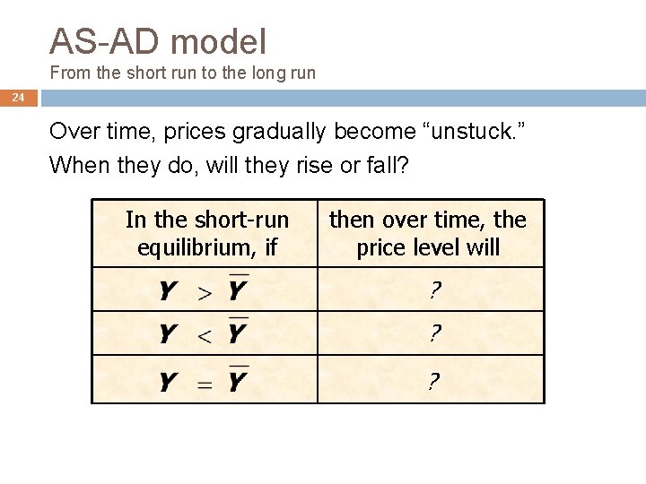
AS-AD model From the short run to the long run 24 Over time, prices gradually become “unstuck. ” When they do, will they rise or fall? In the short-run equilibrium, if then over time, the price level will ? ? ?

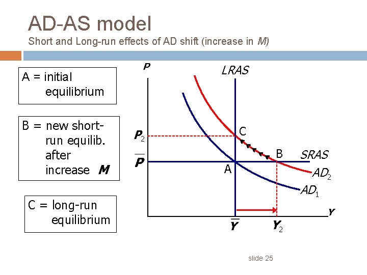
AD-AS model Short and Long-run effects of AD shift (increase in M) A = initial equilibrium B = new shortrun equilib. after increase M C = long-run equilibrium P LRAS C P 2 B A Y 2 slide 25 SRAS AD 2 AD 1 Y

AD-AS model Summary of basic model 26 Bad news – recessions are inevitable Good news – hope for adjustment BUT!!! Reality strikes back Money supply changes are predictable (CB), however, other shocks may shift both curves – unpredictable and even simultaneous Adjustment takes a long time – do we need “nudge” from government?

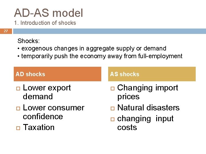
AD-AS model 1. Introduction of shocks 27 Shocks: • exogenous changes in aggregate supply or demand • temporarily push the economy away from full-employment AD shocks Lower export demand Lower consumer confidence Taxation AS shocks Changing import prices Natural disasters changing input costs

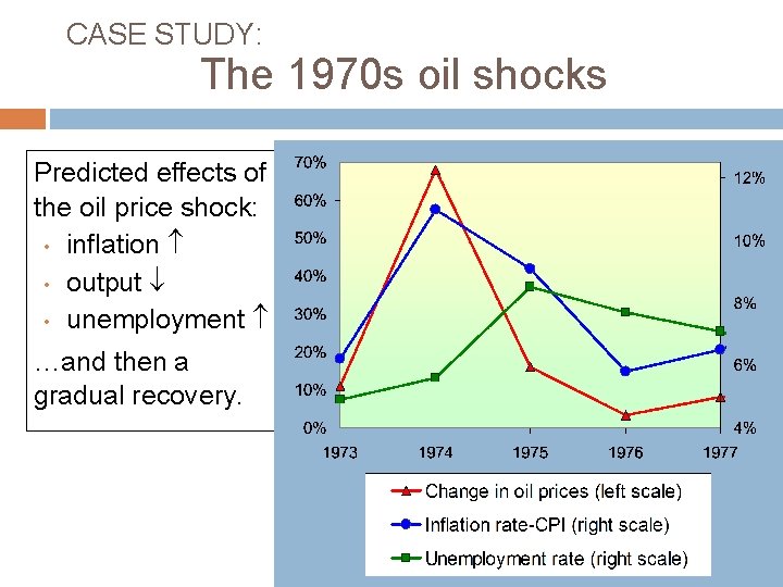
CASE STUDY: The 1970 s oil shocks Early 1970 s: OPEC coordinates a reduction in the supply of oil. Oil prices rose 11% in 1973 68% in 1974 16% in 1975 Such sharp oil price increases are supply shocks because they significantly impact production costs and prices. Q 1: How would this situations look depicted in AD-AS framework?

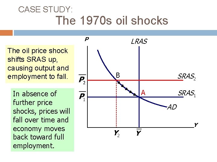
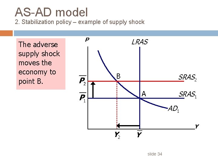
CASE STUDY: The 1970 s oil shocks P The oil price shock shifts SRAS up, causing output and employment to fall. In absence of further price shocks, prices will fall over time and economy moves back toward full employment. LRAS B SRAS 2 SRAS 1 A AD Y 2 Y

CASE STUDY: The 1970 s oil shocks Predicted effects of the oil price shock: • inflation • output • unemployment …and then a gradual recovery.

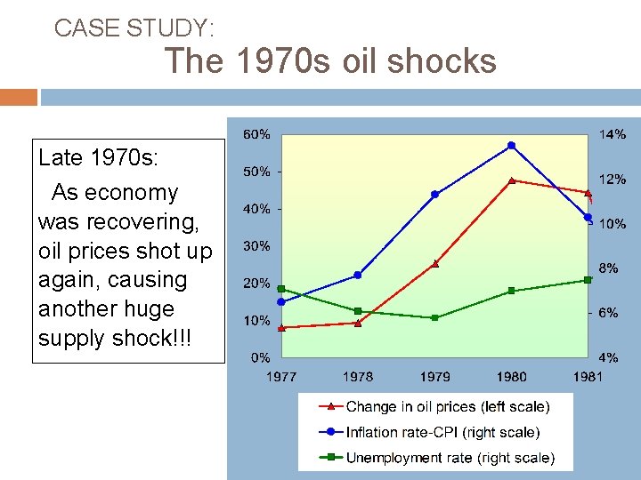
CASE STUDY: The 1970 s oil shocks Late 1970 s: As economy was recovering, oil prices shot up again, causing another huge supply shock!!!

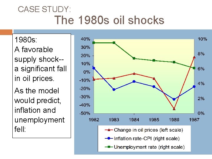
CASE STUDY: The 1980 s oil shocks 1980 s: A favorable supply shock-a significant fall in oil prices. As the model would predict, inflation and unemployment fell:

AS-AD model 2. Stabilization policy 33 Definition: policy actions aimed at reducing the severity of short run economic fluctuations Types: Laissez faire – no action, economy will self-adjust to optimal position Fiscal policy: gvt expenditures, taxation (AD side) Monetary policy: money supply and interest rates Fiscal multiplier Money multiplier Supply side policy: incentives for work, saving, investment Trade policy: e. g. reducing trade barriers

AS-AD model 2. Stabilization policy – example of supply shock The adverse supply shock moves the economy to point B. P LRAS B SRAS 2 SRAS 1 A AD 1 Y Y 2 slide 34

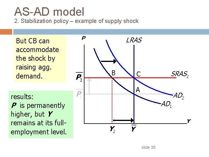
AS-AD model 2. Stabilization policy – example of supply shock But CB can accommodate the shock by raising agg. demand. results: P is permanently higher, but Y remains at its fullemployment level. P LRAS B SRAS 2 C A AD 1 AD 2 Y Y 2 slide 35

AD-AS model Stabilization policy - concerns 36 Which type of policy tool is optimal? What would be the final result? Can we account for all the injections (multiplication) and leakages? How do we account for changing expectations? How do we trade between inflation and unemployment?