Unit 5 Regression Regression line line that minimizes

Unit 5: Regression

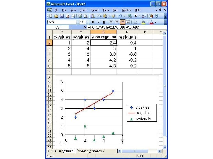
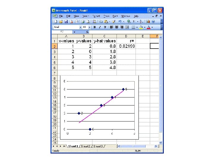
Regression line • line that minimizes sum of squares of vertical distances from data pts (“residuals” or “residues”) • goes through “pt of avgs” ( x , y ) with slope b = r (σy / σx) – by pt-slope: y - y = r (σy / σx)(x - x ) – [so (y-)intercept is y – b x ]

The residuals can show … • nonlinear associations • “heteroscedasticity” – different spreads within vertical slices • [vs. “homoscedastic” – about same SD in slices – not the same range • because slices at different distances from x-avg have diff #s of pts] • So plot’em.

Psych Dept’s version • Regression line is zy = r zx – i. e. , change in x by 1 std unit changes y by the fraction r std unit. • Algebraically equivalent: – (y - y) / σy = r (x - x ) / σx – y - y = r (σy / σx)(x - x )

Projecting y from x with regression • (In business, regression line is “trendline”) • Ex: Cups of coffee and tea drunk daily by CU students. – c = 3, σc = 1, t = 2. 5, σt =. 7, r = -. 4 – If a student drinks 2 coffee, guess how many tea she drinks. • Sol 1: Regr line t - 2. 5 = -. 4(. 7/1)(c - 3), so when c = 2, t = -. 28(2 -3)+2. 5 ≈ 2. 8 • Sol 2: c = 2 in std units is (2 -3)/1 = -1, so project t in std units as -. 4(-1) =. 4, or in cups, . 4(. 7)+2. 5 ≈ 2. 8.

Predictions using regression (II) • Ex: Baldness study, avg # hair (in 10 Ks) is 40, σ = 15; ages avg 36, σ = 20; r = -0. 3. Eqn of regr line? Guess # hair for someone of age 45. . with age 21. • Ex: Admissions Dept guesses 1 st sem GPA (avg 2. 5, σ = 1) from SAT (avg 1200, σ = 200); r = 0. 3. Guess (backward!) SAT for student with 1 st sem GPA 3. 2.

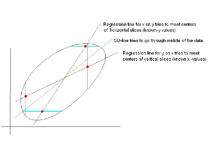
There are 2 regression lines! • Order of variables is now important: • Projecting (guessing) y from x : described above – “regression line of y on x” • Projecting (guessing) x from y : similar formula, but reversing x and y – “regression line of x on y” – graph of this line is more vertical (closer to vertical axis), even more than SD-line – Don’t use the first eqn, substitute y-value and solve for x!

Ex: Which regr line? • College admissions officer uses SAT scores to project 1 st sem GPA: s = 1200, σs = 200, g = 2. 5, σg = 1, r =. 3 – Regression line for g on s: g – 2. 5 =. 3(1/200)(s – 1200) or g =. 0015 s +. 7 • If a student has 1 st sem GPA of 3. 2, what should we guess her SAT is? – (3. 2 -. 7)/. 0015 ≈ 1670? – 1242, from other regr line?

Regression effect • (0<r<1) If we look only at x-values above x, the corresponding y-values will be lower (i. e. , closer to y), –. . . while if we look only at x-values below x, the corresponding y-values will be higher. • Sir Francis Galton (1822 -1911): “regression to mediocrity” • Hence “regression”, though not much is “going back”. • The “regression fallacy” is to attribute this to anything other than imperfect regression. – E. g. , “sophomore slump”

Exs: Regression effect • Comparing results on first and second quizzes: q 1 = 7. 9, σ1 = 1. 8, q 2 = 7. 5, σ2 = 2. 1, r =. 7 – If Fanny got a 10 on first, what should you predict she’ll get on second? – If Fred got 4 on first, what should you guess he’ll get on second? • Parent’s and child’s weights, both at age 40: p = 160, σp = 40, c = 170, σc = 30, r =. 6 – If parent weighed 180 at age 40, what should we guess child will weigh at age 40? – If parent weighed 130, . . .

Projecting %iles with regression • (Assumes both variables are normal, . . . • but avgs and std devs aren’t needed) • Suppose # of hairs on a man’s head and his IQ have r = -. 7: (a) If he is at 80 th %ile in # hairs, about what is his IQ %ile? (b) If he is at 10 th %ile in IQ, about what is hair %ile?

Normal table z Area(%) z Area(%) 0. 0 0. 9 63. 19 1. 8 92. 81 2. 7 99. 31 3. 6 99. 968 0. 05 3. 99 0. 95 65. 79 1. 85 93. 57 2. 75 99. 4 3. 65 99. 974 0. 1 7. 97 1 68. 27 1. 9 94. 26 2. 8 99. 49 3. 7 99. 978 0. 15 11. 92 1. 05 70. 63 1. 95 94. 88 2. 85 99. 56 3. 75 99. 982 0. 2 15. 85 1. 1 72. 87 2 95. 45 2. 9 99. 63 3. 8 99. 986 0. 25 19. 74 1. 15 74. 99 2. 05 95. 96 2. 95 99. 68 3. 85 99. 988 0. 3 23. 58 1. 2 76. 99 2. 1 96. 43 3 99. 73 3. 9 99. 99 0. 35 27. 37 1. 25 78. 87 2. 15 96. 84 3. 05 99. 771 3. 95 99. 992 0. 4 31. 08 1. 3 80. 64 2. 2 97. 22 3. 1 99. 806 4 99. 9937 0. 45 34. 73 1. 35 82. 3 2. 25 97. 56 3. 15 99. 837 4. 05 99. 9949 0. 5 38. 29 1. 4 83. 85 2. 3 97. 86 3. 2 99. 863 4. 1 99. 9959 0. 55 41. 77 1. 45 85. 29 2. 35 98. 12 3. 25 99. 885 4. 15 99. 9967 0. 6 45. 15 1. 5 86. 64 2. 4 98. 36 3. 3 99. 903 4. 2 99. 9973 0. 65 48. 43 1. 55 87. 89 2. 45 98. 57 3. 35 99. 919 4. 25 99. 9979 0. 7 51. 61 1. 6 89. 04 2. 5 98. 76 3. 4 99. 933 4. 3 99. 9983 0. 75 54. 67 1. 65 90. 11 2. 55 98. 92 3. 45 99. 944 4. 35 99. 9986 0. 8 57. 63 1. 7 91. 09 2. 6 99. 07 3. 5 99. 953 4. 4 99. 9989 0. 85 60. 47 1. 75 91. 99 2. 65 99. 2 3. 55 99. 961 4. 45 99. 9991

RMS error for regression • This is the square root of the average of the squares of the residues, i. e. , the differences between the y-values of the data points and the y-values on the regression line (predictions) at the same x-values. • Also called “residual standard error” • Regr line was chosen to minimize this value • Using formula for regr line (and a lot of algebra), we find this is just σy √[1 -r 2] – Note formula uses the σ of the variable we are trying to project

Rule of thumb for regression • About 68% of the data pts will be within 1 RMS error for regr of the regr line; about 95% within 2 • √[1 -r 2] < 1, so this rule gives a thinner, sloping swath covering 68% (or 95%) of data pts than the original thicker, horizontal swath

If the data is homoscedastic, • i. e. , std devs in vertical slices of data are roughly equal throughout • (text calls this “football-shaped”, but “cigar-shaped” would be just as sensible, depending on relative sizes of σx , σy ), . . . • then RMS error for regr is this common σ. • Ex: SAT scores vs. 1 st sem GPA: s = 1200, σs = 200, g = 2. 5, σg = 1, r =. 3 – – Project GPA if SAT is 1300 by regr: 2. 65 Likely to be off by RMS error: 1√[1 -. 32] ≈. 95 If GPA is 1. 8, guess SAT by regr: 1158 Likely to be off by 200√[1 -. 32] ≈ 191

Normal approx within a vertical slice (? ? ? ) • Ex (cntd): SAT scores vs. 1 st sem GPA: s = 1200, σs = 200, g = 2. 5, σg = 1, r =. 3 • (and assume homoscedastic): • Suppose a student has a 1300 SAT and a 3. 7 GPA. What %ile does that make her GPA among the students who got 1300 SATs? – In that group (like all the other vertical slices), best guess for σ is RMS error for regr, ≈. 95, – and by regr, best guess for avg within slice is 2. 65, – so in slice, her GPA z-value is (3. 7 -2. 65)/. 95 ≈ 1. 10 – and by normal table, that’s 86 th %ile

Warning on regression: • Don’t extrapolate. • Ex: Grade inflation at CU: GPA avg in F 1993 was 2. 91, increasing 0. 008/sem (r = 0. 93). By S 2058, avg GPA will be 4. 00. (? )

HERE BE DRAGONS • From this point on in this presentation, the material is not in the text. • In fact, our authors specifically warn against some methods (like transforming data), but the methods are commonly used. • This material will not be on an exam, . . . • but multivariate regression is used in Midterm Project II.

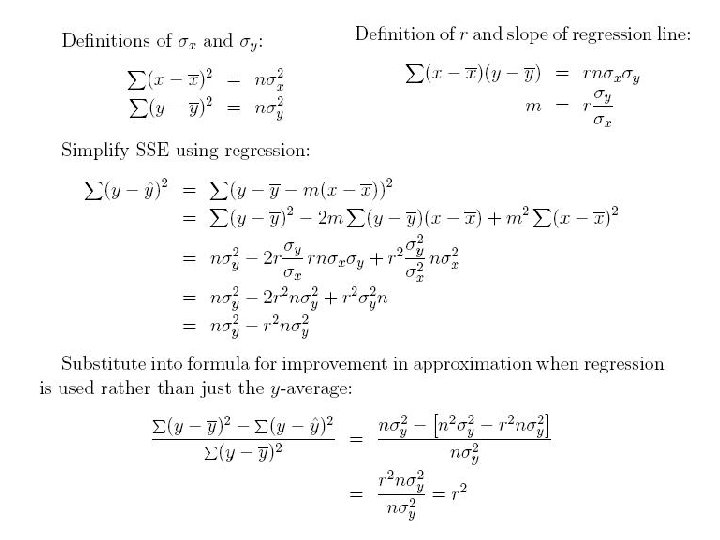
What does r 2 measure? • Answer: It says how much better for predicting y is using regr line (i. e. , using the y-value ŷ on the regression line at that point) than just always using y – Difference of SSE (sum of squares of errors) using avg [i. e. , ∑(y - y)2] vs. SSE using regr [i. e. , sum of squares of residuals ∑(y - ŷ)2], divided by SSE using avg. . . –. . . which = r 2 (see next slide) – so, if r 2 = 0. 4, say, “regression results in a 40% improvement in projection”

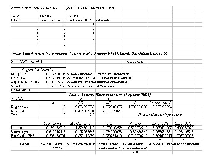
Multiple (linear) regression • If there is more than one explanatory variable (x 1, x 2, x 3 say) and one response variable (y), it may be useful to model it as y = a + b 1 x 1 + b 2 x 2 + b 3 x 3 • Ex: Aspirin is so acidic that it often upsets the stomach, so it is often administered with an antacid -- which limits effect. Suppose the pain, measured by the rating of headache sufferers, is given by p = 5 -. 3 s +. 2 t where s is the aspirin dose and t is the antacid dose.

Graphs of aspirin example

Multiple regression • As with simple regression, there is a (multiple) correlation R (indep of units) that measures how closely the data points (in 3 -space or higher dims) follow a (hyper)plane • (What does the sign mean, because y can go up when x 1 goes up or when x 2 goes down? ) • In this case R 2 is easier to understand (and means the same as before), so it appears in the computer outputs as well • The next page is Excel output from a (fictional) economic multiple. (Bold italics = added)

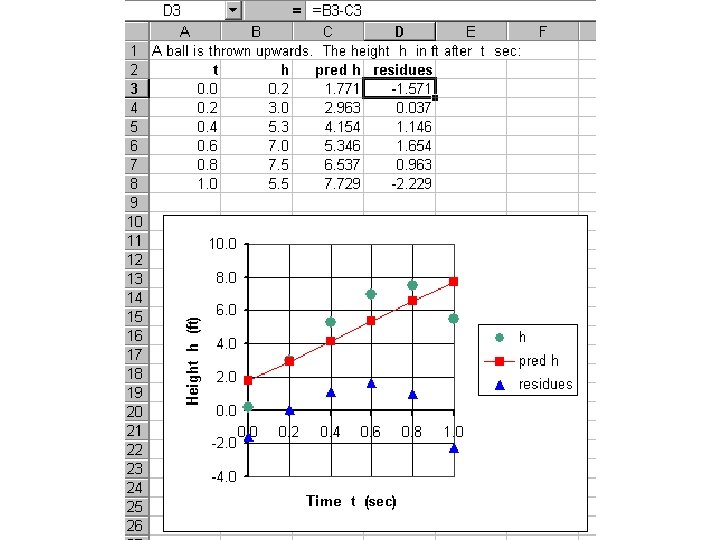
Polynomial regression • If theory or scatterplot (or plot of residues) suggests a higher-degree polynomial would fit data better than linear regression of y on x , add cols of x 2 (and x 3 and. . . ) and do multiple regression. • Ex of theory: path of projectile under gravity, weight vs. height • Ex of fitting: Boston poverty level vs. property values (Midterm Project I)

Model with Y = p. A + q. B + r. AB ?

Correlations in multiple regression • If we add more x-variables in an attempt to approximate a y-variable, the absolute R-value (or R 2 -value) cannot go down. – It will probably go up, unless there is no relation at all between the new x-variables and y. • But the correlations between the old x-variables and y may change – may even change sign! – as new x -values are added. – Ex: In the thrown ball example, both t 2 and h go up, at least initially, so without t their correlation is positive. But if we add t , it’s a better determiner of h , and t 2 becomes a negative influence on h, namely in the gravity term.

Curvilinear associations • (Linear) regression, as we have studied it, is built to find the best line approximating data. But sometimes theory, or just a curviness of the data cloud, hint that the equation that best relates the xand y-values is not a line. • In this case, experimenters often “transform” the data, replacing the x-, or y-, or both values by their logs, or their squares, or. . . and use regression on the new data to find slopes and intercepts, which translate to exponents or other constants in equations for the original data • The next few slides are a fast intro to some common forms of equations that might relate variables.

Exponential regression • In many situations, an exponential function fits data better than a linear one. – population – radioactive decay • Form: y = a bx for some constants a, b

Logarithms • • y = bx and x = logb(y) say the same thing From cxcy = cx+y : logc(uv) = logc(u) + logc(v) From (cy)x = cyx : logc(ax) = x logc(a) So y = a bx can be written as logc(y) = logc(a) + x logc(b) • Thus, x and logc(y) are linearly related • So maybe replace (“transform”) y by logc(y) – (Our authors don’t trust this or any other transformation, because any measurement errors, which were originally assumed normally distributed, won’t remain so after the transformation)

Richter

Exp and log notation • e = 2. 71828. . . (more convenient base for calculus reasons) • exp(x) = ex – [Note: ax = (blogb(a))x = bx logb(a) – so switching bases is just a linear change of variable (sorta)] • ln = loge ; log = log 10 , log 2 , . . .

Logistic models • Several applications fit “logistic” models better than linear, exp or log – y = K ea+bx/(1+ea+bx) – For large x , y is close to K • In population models, K is “carrying capacity”, i. e. , max sustainable pop • But y may be proportion p of pop, so K=1 – For large neg x , y is close to 0 • Ex: Smokers: x = # packs/day, p = % who smoke that much and have a cough

For logistic with K = 1, . . . • x and ln(y/(1 -y)) are related linearly: – y = ea+bx / (1 + ea+bx) – y + yea+bx = ea+bx – yea+bx = (1 -y)ea+bx – y/(1 -y) = ea+bx – ln(y/(1 -y)) = a+bx • so maybe “transform” y to ln(y/(1 -y))