Unit 6 Regression What is regression Regression Tendency

Unit 6 Regression

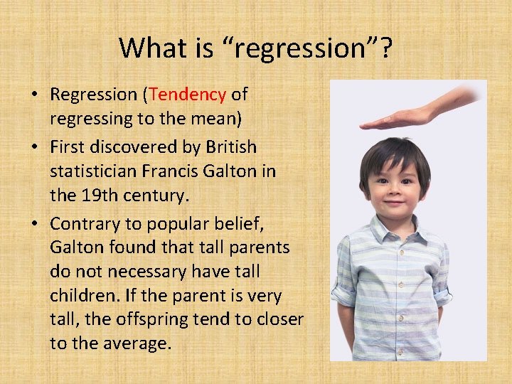
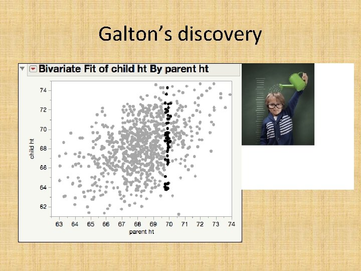
What is “regression”? • Regression (Tendency of regressing to the mean) • First discovered by British statistician Francis Galton in the 19 th century. • Contrary to popular belief, Galton found that tall parents do not necessary have tall children. If the parent is very tall, the offspring tend to closer to the average.

Galton’s discovery

Difference between correlation and regression • In correlation there is no distinction between DV and IV. • Correlation doesn’t necessarily imply causation. • Correlation of X and Y = Correlation of Y and X • Regression of Y by X is NOT the same as regression of X by Y. • In regression Y is the DV and X is the IV. The model may imply a cause and effect relationship.

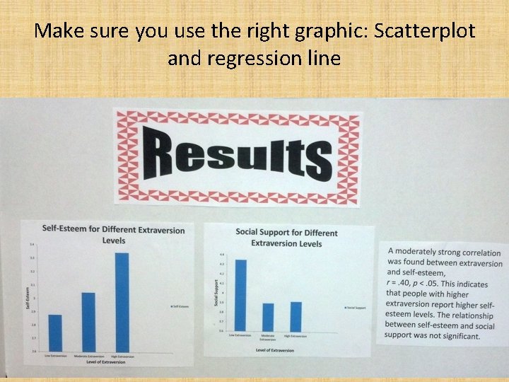
Make sure you use the right graphic: Scatterplot and regression line

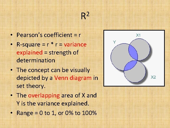
R 2 • Pearson’s coefficient = r • R-square = r * r = variance explained = strength of determination • The concept can be visually depicted by a Venn diagram in set theory. • The overlapping area of X and Y is the variance explained. • Range = 0 to 1, or 0% to 100%

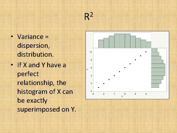
R 2 • Variance = dispersion, distribution. • If X and Y have a perfect relationship, the histogram of X can be exactly superimposed on Y.

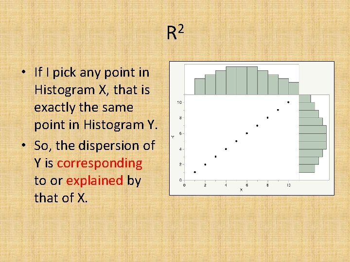
R 2 • If I pick any point in Histogram X, that is exactly the same point in Histogram Y. • So, the dispersion of Y is corresponding to or explained by that of X.

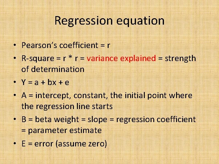
Regression equation • Pearson’s coefficient = r • R-square = r * r = variance explained = strength of determination • Y = a + bx + e • A = intercept, constant, the initial point where the regression line starts • B = beta weight = slope = regression coefficient = parameter estimate • E = error (assume zero)

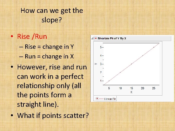
How can we get the slope? • Rise /Run – Rise = change in Y – Run = change in X • However, rise and run can work in a perfect relationship only (all the points form a straight line). • What if points scatter?

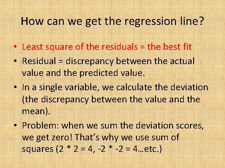
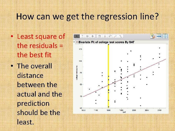
How can we get the regression line? • Least square of the residuals = the best fit • Residual = discrepancy between the actual value and the predicted value. • In a single variable, we calculate the deviation (the discrepancy between the value and the mean). • Problem: when we sum the deviation scores, we get zero! That’s why we use sum of squares (2 * 2 = 4, -2 * -2 = 4…etc. )

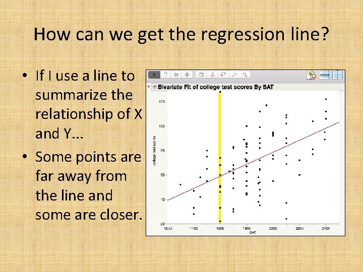
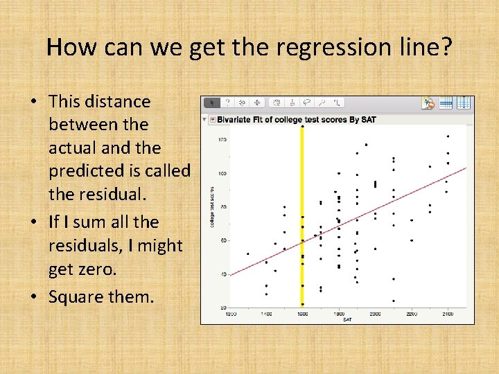
How can we get the regression line? • If I use a line to summarize the relationship of X and Y. . . • Some points are far away from the line and some are closer.

How can we get the regression line? • This distance between the actual and the predicted is called the residual. • If I sum all the residuals, I might get zero. • Square them.

How can we get the regression line? • Least square of the residuals = the best fit • The overall distance between the actual and the prediction should be the least.

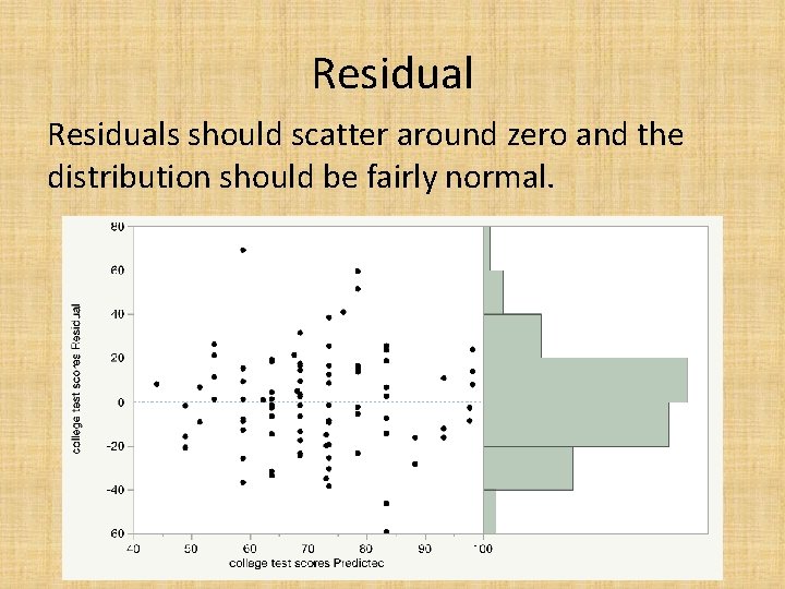
Residuals should scatter around zero and the distribution should be fairly normal.

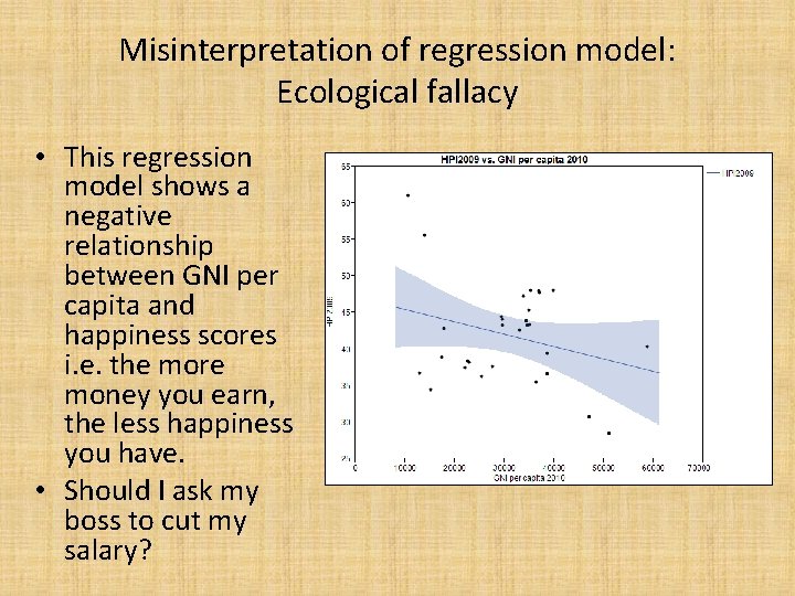
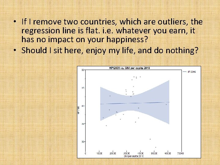
Misinterpretation of regression model: Ecological fallacy • This regression model shows a negative relationship between GNI per capita and happiness scores i. e. the more money you earn, the less happiness you have. • Should I ask my boss to cut my salary?

• If I remove two countries, which are outliers, the regression line is flat. i. e. whatever you earn, it has no impact on your happiness? • Should I sit here, enjoy my life, and do nothing?

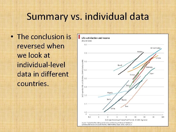
Summary vs. individual data • The conclusion is reversed when we look at individual-level data in different countries.

Using summary data to infer to individuals • Another well-known example is the report of Wall Street Journal (June 22, 1995) showing a negative relationship between the rank of each state's average SAT score and average expenditure on education. At first glance it implies that spending less on education will improve SAT scores. – Cost of living and expenditures vary from state to state. – Not everyone takes the SAT. Some take ACT.

NAEP • When we examine the achievement data from the National Assessment of Education Progress (NAEP) based on a representative sample, it was found that there is a positive relationship between NAEP and expenditures.

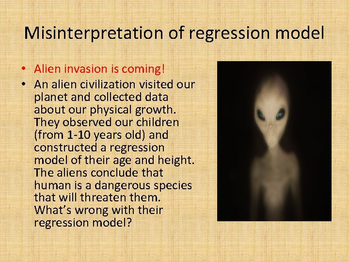
Misinterpretation of regression model • Alien invasion is coming! • An alien civilization visited our planet and collected data about our physical growth. They observed our children (from 1 -10 years old) and constructed a regression model of their age and height. The aliens conclude that human is a dangerous species that will threaten them. What’s wrong with their regression model?

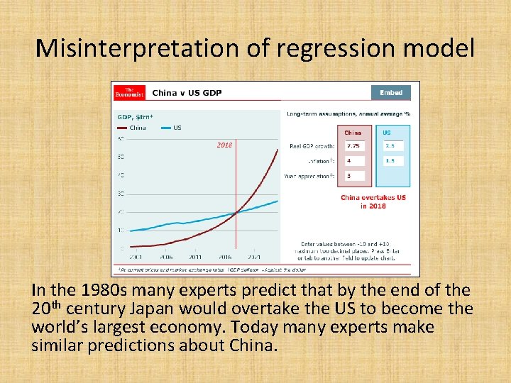
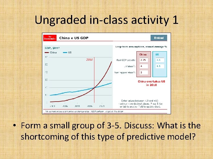
Misinterpretation of regression model In the 1980 s many experts predict that by the end of the 20 th century Japan would overtake the US to become the world’s largest economy. Today many experts make similar predictions about China.

Ungraded in-class activity 1 • Form a small group of 3 -5. Discuss: What is the shortcoming of this type of predictive model?

Black swan vs. Elephant in the room • The book entitled "The Signal and the Noise" by Nate Silver also used the collapse of Japan in the early 1990 s as an example. The bloom of Japan in the 1980 s was unrealistic because the real estate price could not go up forever. • Before 2008 the majority of the US experts could not predict a crash like that of Japan would happen in the US. But Silver asserted that the 2008 crash is not a Black Swan; rather, it is an elephant in the room. • It was right there, but no one saw it or refused to see it. Nothing could keep rising forever!

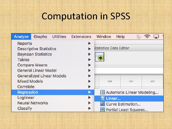
Computation in SPSS

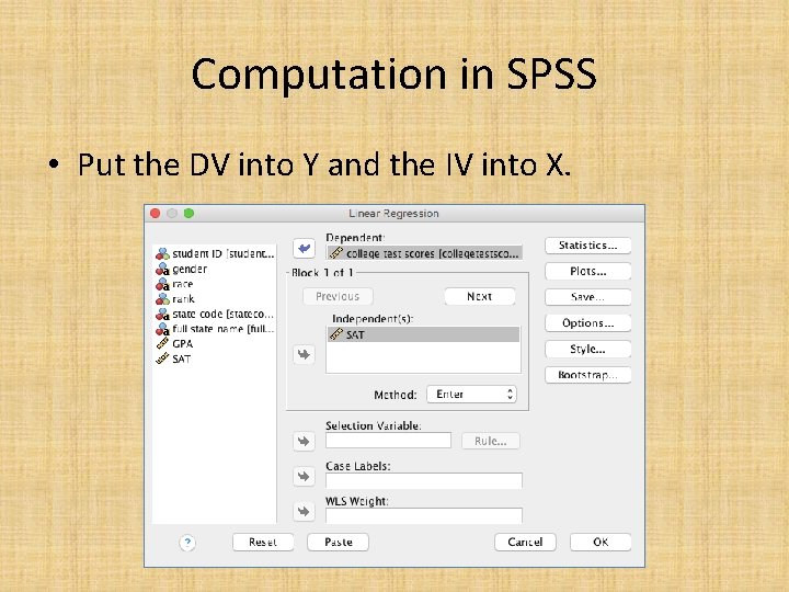
Computation in SPSS • Put the DV into Y and the IV into X.

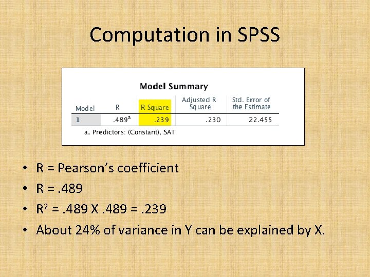
Computation in SPSS • • R = Pearson’s coefficient R =. 489 R 2 =. 489 X. 489 =. 239 About 24% of variance in Y can be explained by X.

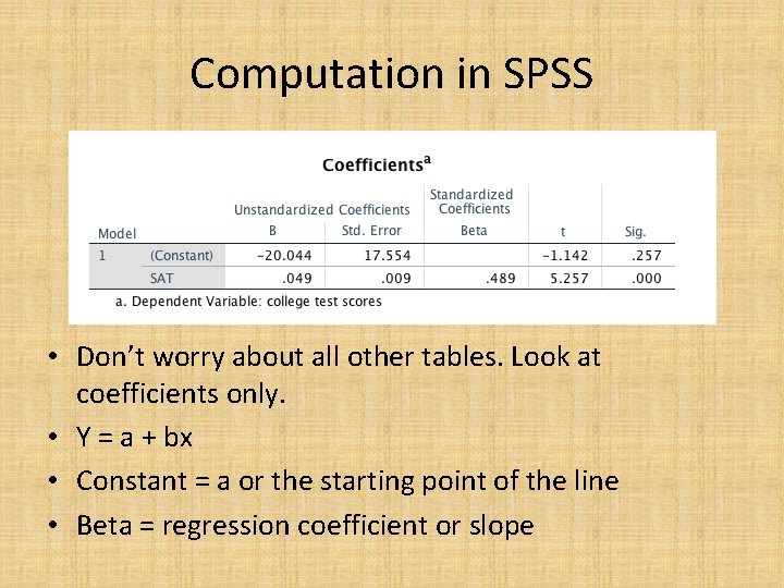
Computation in SPSS • Don’t worry about all other tables. Look at coefficients only. • Y = a + bx • Constant = a or the starting point of the line • Beta = regression coefficient or slope

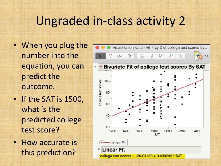
Ungraded in-class activity 2 • When you plug the number into the equation, you can predict the outcome. • If the SAT is 1500, what is the predicted college test score? • How accurate is this prediction?

Assignment 6 (Canvas) • Use the data set “visualization_data” to run a simple regression model. • Model 1: Use college test scores as the dependent variable (Y) and GPA as the independent variable (X). What is the regression equation (y = a + bx)? • Model 2: Use GPA as the DV and college test scores as the IV. What is the regression equation now? • Is regression of Y by X the same as regression of X by Y?