SQL 2018 Fall Pusan National University KiJoune Li

SQL 2018, Fall Pusan National University Ki-Joune Li

Why SQL? • SQL very-high-level language o the programmer is able to avoid specifying a lot of datamanipulation details unlike C++ o • What makes SQL viable is that its queries are “optimized” quite well, yielding efficient query executions. • Data Definition • Data Manipulation 2

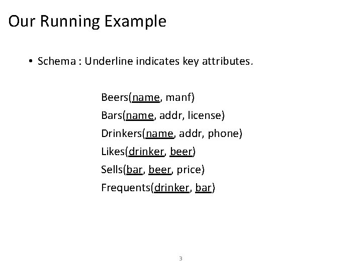
Our Running Example • Schema : Underline indicates key attributes. Beers(name, manf) Bars(name, addr, license) Drinkers(name, addr, phone) Likes(drinker, beer) Sells(bar, beer, price) Frequents(drinker, bar) 3

Data Definition: Defining a Database Schema • A database schema comprises declarations for the relations (“tables”) of the database. • Many other kinds of elements may also appear in the database schema, including views, indexes, and triggers. 4

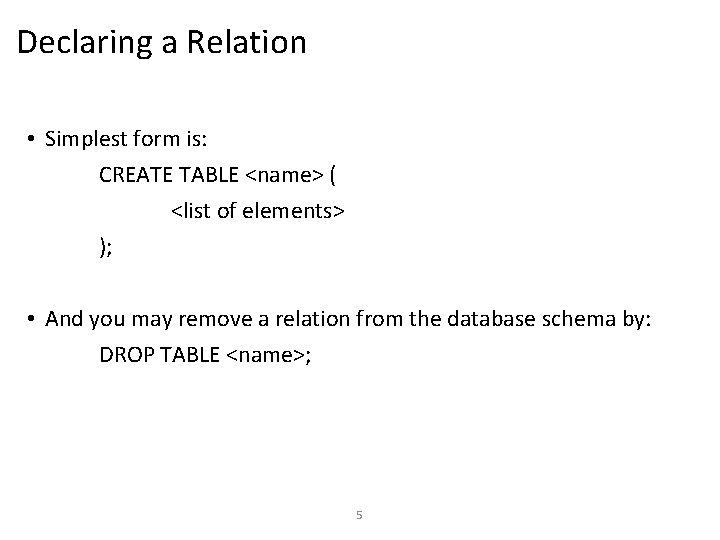
Declaring a Relation • Simplest form is: CREATE TABLE <name> ( <list of elements> ); • And you may remove a relation from the database schema by: DROP TABLE <name>; 5

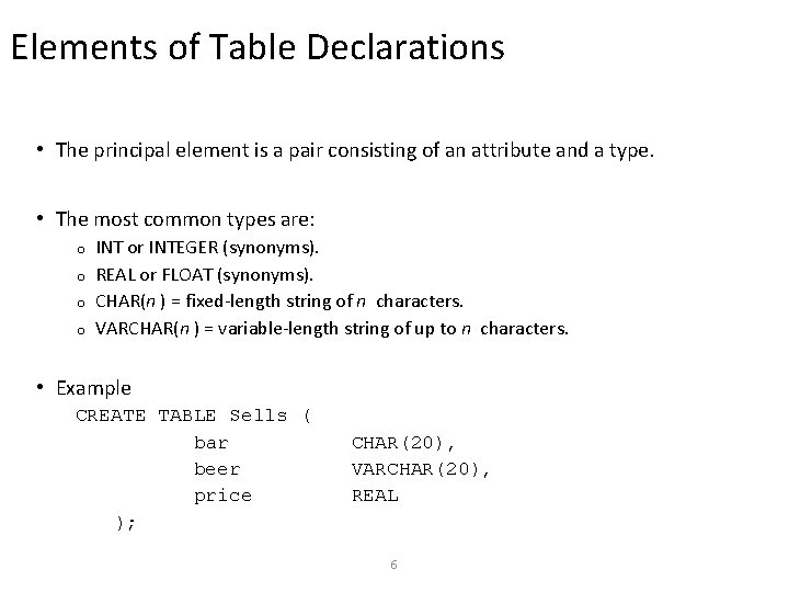
Elements of Table Declarations • The principal element is a pair consisting of an attribute and a type. • The most common types are: INT or INTEGER (synonyms). o REAL or FLOAT (synonyms). o CHAR(n ) = fixed-length string of n characters. o VARCHAR(n ) = variable-length string of up to n characters. o • Example CREATE TABLE Sells ( bar beer price ); CHAR(20), VARCHAR(20), REAL 6

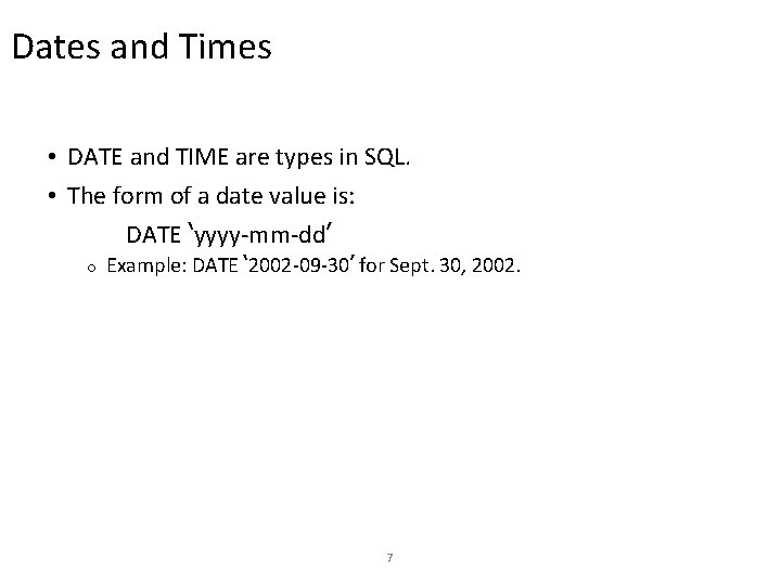
Dates and Times • DATE and TIME are types in SQL. • The form of a date value is: DATE ‘yyyy-mm-dd’ o Example: DATE ‘ 2002 -09 -30’ for Sept. 30, 2002. 7

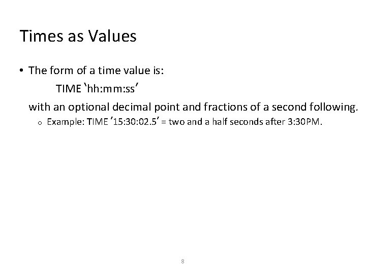
Times as Values • The form of a time value is: TIME ‘hh: mm: ss’ with an optional decimal point and fractions of a second following. o Example: TIME ’ 15: 30: 02. 5’ = two and a half seconds after 3: 30 PM. 8

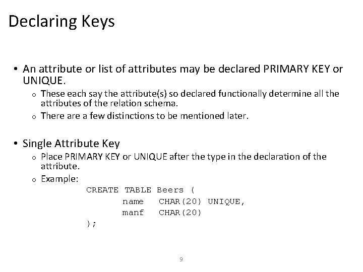
Declaring Keys • An attribute or list of attributes may be declared PRIMARY KEY or UNIQUE. These each say the attribute(s) so declared functionally determine all the attributes of the relation schema. o There a few distinctions to be mentioned later. o • Single Attribute Key Place PRIMARY KEY or UNIQUE after the type in the declaration of the attribute. o Example: o CREATE TABLE Beers ( name CHAR(20) UNIQUE, manf CHAR(20) ); 9

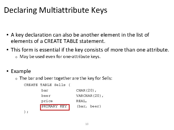
Declaring Multiattribute Keys • A key declaration can also be another element in the list of elements of a CREATE TABLE statement. • This form is essential if the key consists of more than one attribute. o May be used even for one-attribute keys. • Example o The bar and beer together are the key for Sells: CREATE TABLE Sells ( bar beer price PRIMARY KEY ); CHAR(20), VARCHAR(20), REAL, (bar, beer) 10

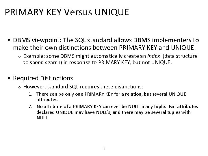
PRIMARY KEY Versus UNIQUE • DBMS viewpoint: The SQL standard allows DBMS implementers to make their own distinctions between PRIMARY KEY and UNIQUE. o Example: some DBMS might automatically create an index (data structure to speed search) in response to PRIMARY KEY, but not UNIQUE. • Required Distinctions o However, standard SQL requires these distinctions: 1. There can be only one PRIMARY KEY for a relation, but several UNIQUE attributes. 2. No attribute of a PRIMARY KEY can ever be NULL in any tuple. But attributes declared UNIQUE may have NULL’s, and there may be several tuples with NULL. 11

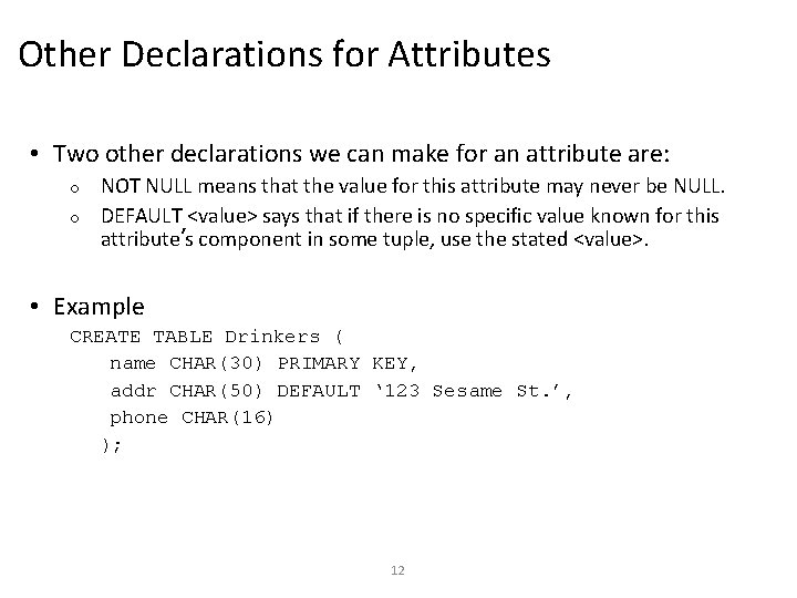
Other Declarations for Attributes • Two other declarations we can make for an attribute are: NOT NULL means that the value for this attribute may never be NULL. o DEFAULT <value> says that if there is no specific value known for this attribute’s component in some tuple, use the stated <value>. o • Example CREATE TABLE Drinkers ( name CHAR(30) PRIMARY KEY, addr CHAR(50) DEFAULT ‘ 123 Sesame St. ’, phone CHAR(16) ); 12

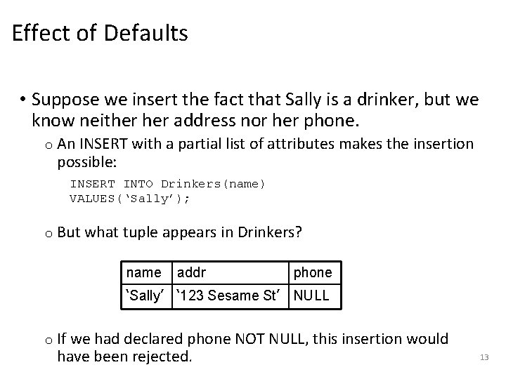
Effect of Defaults • Suppose we insert the fact that Sally is a drinker, but we know neither address nor her phone. o An INSERT with a partial list of attributes makes the insertion possible: INSERT INTO Drinkers(name) VALUES(‘Sally’); o o But what tuple appears in Drinkers? name addr phone ‘Sally’ ‘ 123 Sesame St’ NULL If we had declared phone NOT NULL, this insertion would have been rejected. 13

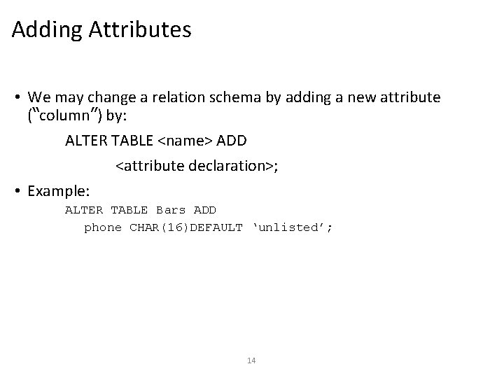
Adding Attributes • We may change a relation schema by adding a new attribute (“column”) by: ALTER TABLE <name> ADD <attribute declaration>; • Example: ALTER TABLE Bars ADD phone CHAR(16)DEFAULT ‘unlisted’; 14

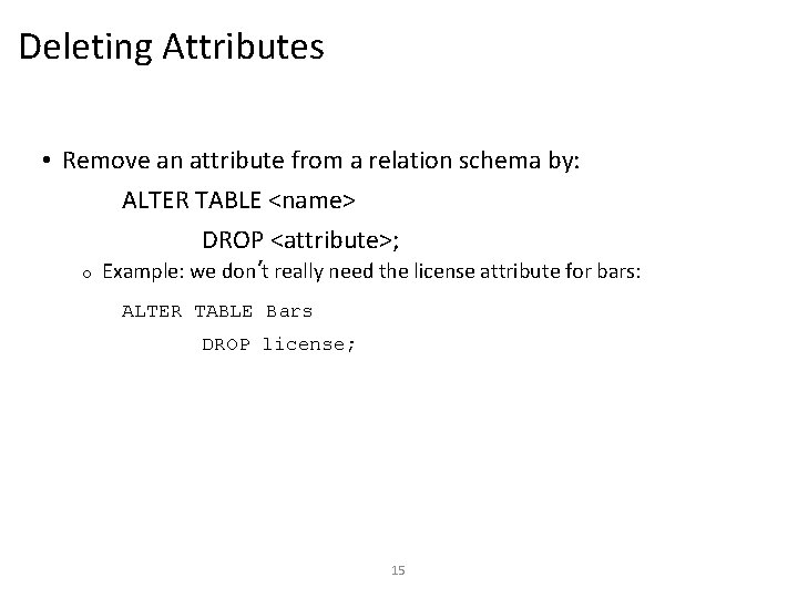
Deleting Attributes • Remove an attribute from a relation schema by: ALTER TABLE <name> DROP <attribute>; o Example: we don’t really need the license attribute for bars: ALTER TABLE Bars DROP license; 15

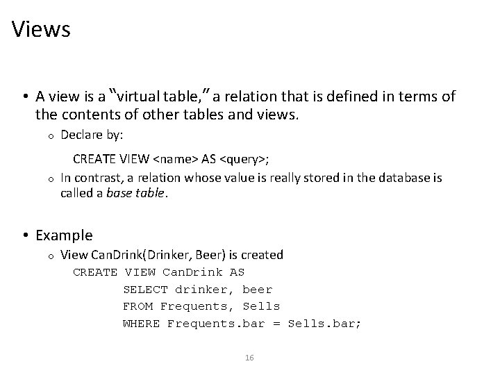
Views • A view is a “virtual table, ” a relation that is defined in terms of the contents of other tables and views. o Declare by: CREATE VIEW <name> AS <query>; o In contrast, a relation whose value is really stored in the database is called a base table. • Example o View Can. Drink(Drinker, Beer) is created CREATE VIEW Can. Drink AS SELECT drinker, beer FROM Frequents, Sells WHERE Frequents. bar = Sells. bar; 16

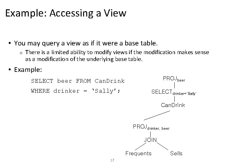
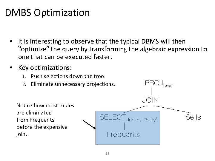
Example: Accessing a View • You may query a view as if it were a base table. o There is a limited ability to modify views if the modification makes sense as a modification of the underlying base table. • Example: PROJbeer SELECT beer FROM Can. Drink WHERE drinker = ‘Sally’; SELECTdrinker=‘Sally’ Can. Drink PROJdrinker, beer JOIN Frequents 17 Sells

DMBS Optimization • It is interesting to observe that the typical DBMS will then “optimize” the query by transforming the algebraic expression to one that can be executed faster. • Key optimizations: Push selections down the tree. 2. Eliminate unnecessary projections. 1. Notice how most tuples are eliminated from Frequents before the expensive join. PROJbeer JOIN SELECTdrinker=‘Sally’ Frequents 18 Sells

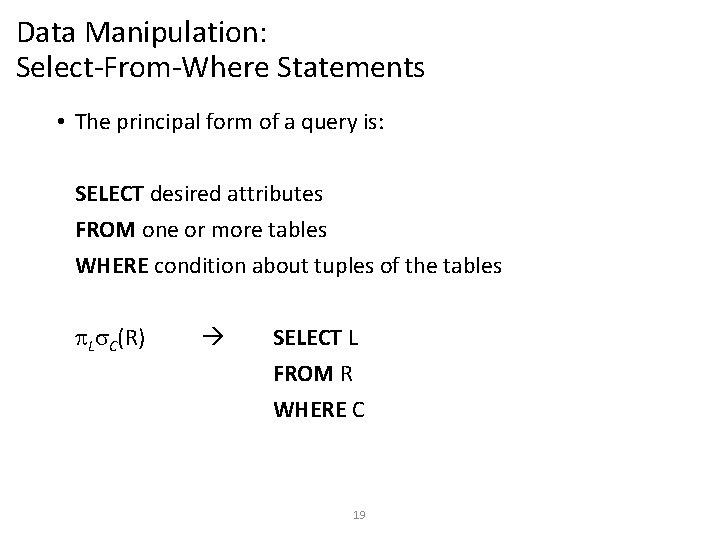
Data Manipulation: Select-From-Where Statements • The principal form of a query is: SELECT desired attributes FROM one or more tables WHERE condition about tuples of the tables p. Ls. C(R) SELECT L FROM R WHERE C 19

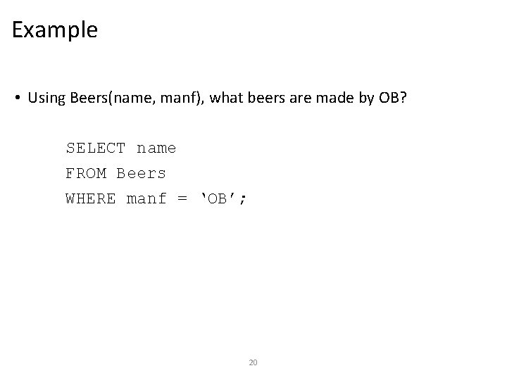
Example • Using Beers(name, manf), what beers are made by OB? SELECT name FROM Beers WHERE manf = ‘OB’; 20

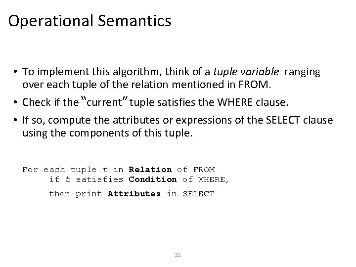
Operational Semantics • To implement this algorithm, think of a tuple variable ranging over each tuple of the relation mentioned in FROM. • Check if the “current” tuple satisfies the WHERE clause. • If so, compute the attributes or expressions of the SELECT clause using the components of this tuple. For each tuple t in Relation of FROM if t satisfies Condition of WHERE, then print Attributes in SELECT 21

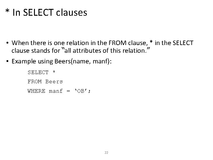
* In SELECT clauses • When there is one relation in the FROM clause, * in the SELECT clause stands for “all attributes of this relation. ” • Example using Beers(name, manf): SELECT * FROM Beers WHERE manf = ‘OB’; 22

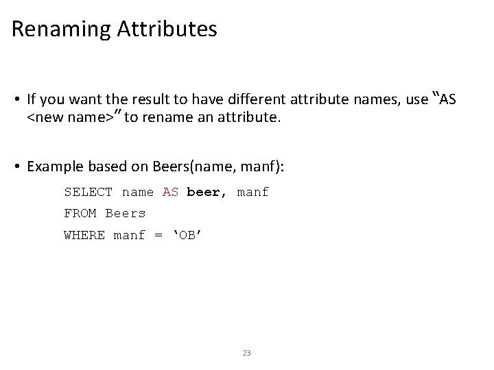
Renaming Attributes • If you want the result to have different attribute names, use “AS <new name>” to rename an attribute. • Example based on Beers(name, manf): SELECT name AS beer, manf FROM Beers WHERE manf = ‘OB’ 23

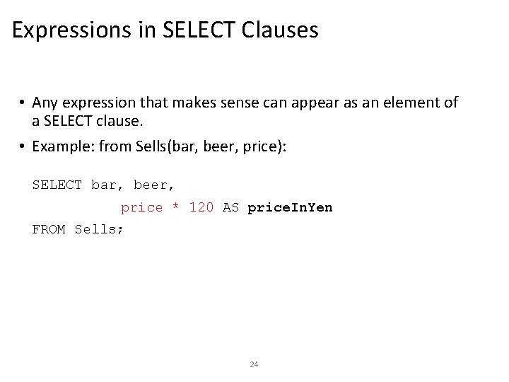
Expressions in SELECT Clauses • Any expression that makes sense can appear as an element of a SELECT clause. • Example: from Sells(bar, beer, price): SELECT bar, beer, price * 120 AS price. In. Yen FROM Sells; 24

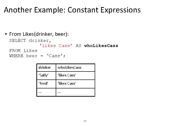
Another Example: Constant Expressions • From Likes(drinker, beer): SELECT drinker, ‘likes Cass’ AS who. Likes. Cass FROM Likes WHERE beer = ‘Cass’; drinker who. Likes. Cass ‘Sally’ ‘likes Cass’ ‘Fred’ ‘likes Cass’ . . . 25

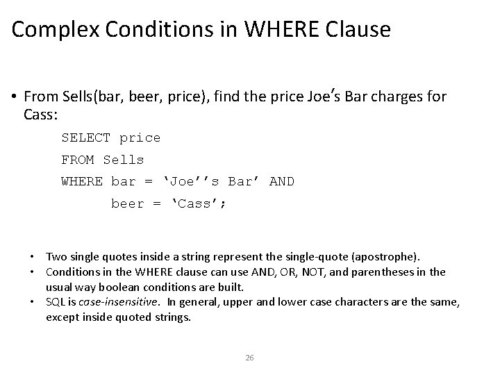
Complex Conditions in WHERE Clause • From Sells(bar, beer, price), find the price Joe’s Bar charges for Cass: SELECT price FROM Sells WHERE bar = ‘Joe’’s Bar’ AND beer = ‘Cass’; • Two single quotes inside a string represent the single-quote (apostrophe). • Conditions in the WHERE clause can use AND, OR, NOT, and parentheses in the usual way boolean conditions are built. • SQL is case-insensitive. In general, upper and lower case characters are the same, except inside quoted strings. 26

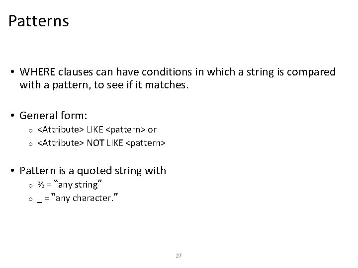
Patterns • WHERE clauses can have conditions in which a string is compared with a pattern, to see if it matches. • General form: <Attribute> LIKE <pattern> or o <Attribute> NOT LIKE <pattern> o • Pattern is a quoted string with % = “any string” o _ = “any character. ” o 27

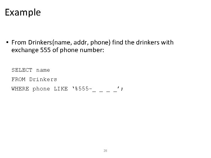
Example • From Drinkers(name, addr, phone) find the drinkers with exchange 555 of phone number: SELECT name FROM Drinkers WHERE phone LIKE ‘%555 -_ _ _ _’; 28

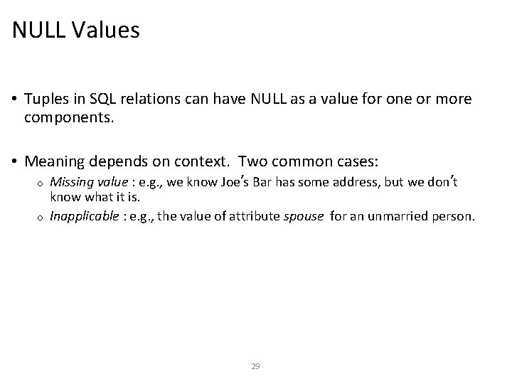
NULL Values • Tuples in SQL relations can have NULL as a value for one or more components. • Meaning depends on context. Two common cases: Missing value : e. g. , we know Joe’s Bar has some address, but we don’t know what it is. o Inapplicable : e. g. , the value of attribute spouse for an unmarried person. o 29

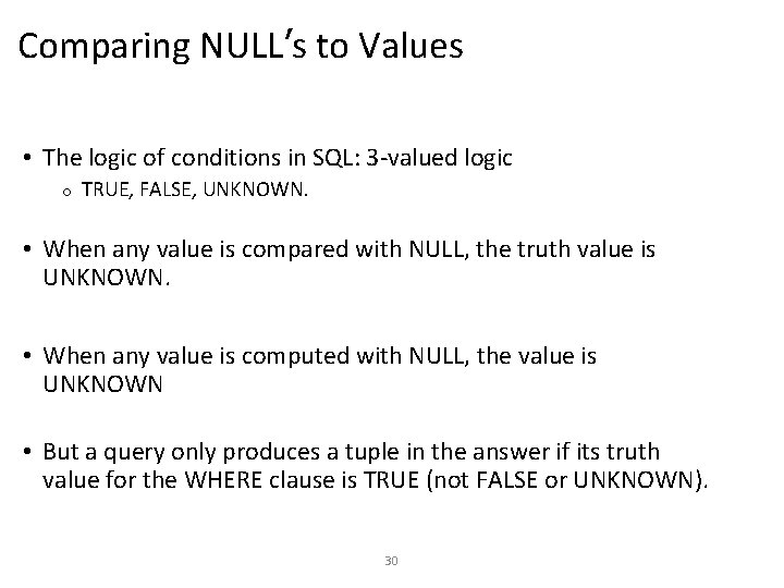
Comparing NULL’s to Values • The logic of conditions in SQL: 3 -valued logic o TRUE, FALSE, UNKNOWN. • When any value is compared with NULL, the truth value is UNKNOWN. • When any value is computed with NULL, the value is UNKNOWN • But a query only produces a tuple in the answer if its truth value for the WHERE clause is TRUE (not FALSE or UNKNOWN). 30

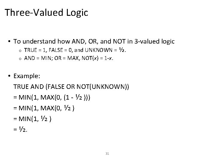
Three-Valued Logic • To understand how AND, OR, and NOT in 3 -valued logic TRUE = 1, FALSE = 0, and UNKNOWN = ½. o AND = MIN; OR = MAX, NOT(x) = 1 -x. o • Example: TRUE AND (FALSE OR NOT(UNKNOWN)) = MIN(1, MAX(0, (1 - ½ ))) = MIN(1, MAX(0, ½ ) = MIN(1, ½ ) = ½. 31

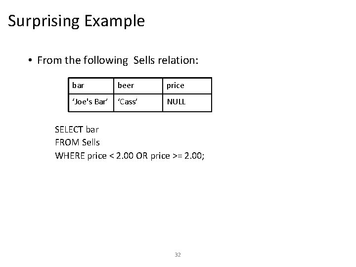
Surprising Example • From the following Sells relation: bar beer price ‘Joe's Bar’ ‘Cass’ NULL SELECT bar FROM Sells WHERE price < 2. 00 OR price >= 2. 00; 32

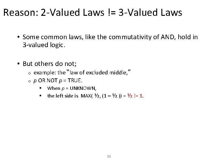
Reason: 2 -Valued Laws != 3 -Valued Laws • Some common laws, like the commutativity of AND, hold in 3 -valued logic. • But others do not; example: the “law of excluded middle, ” o p OR NOT p = TRUE. o § § When p = UNKNOWN, the left side is MAX( ½, (1 – ½ )) = ½ != 1. 33

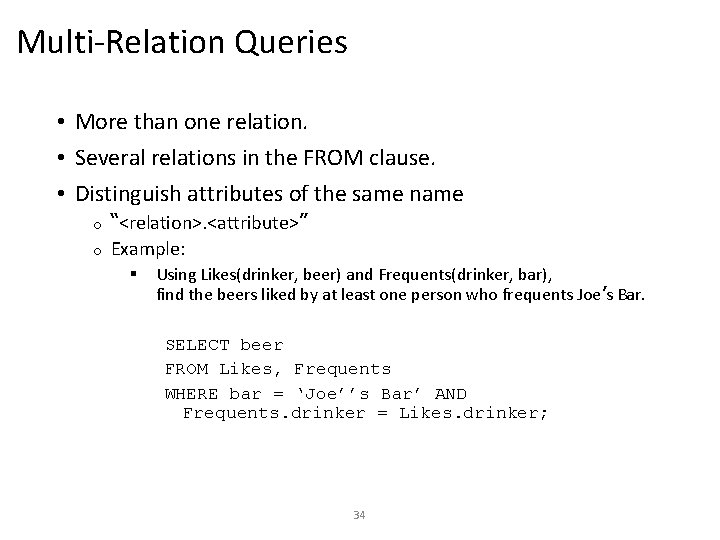
Multi-Relation Queries • More than one relation. • Several relations in the FROM clause. • Distinguish attributes of the same name “<relation>. <attribute>” o Example: o § Using Likes(drinker, beer) and Frequents(drinker, bar), find the beers liked by at least one person who frequents Joe’s Bar. SELECT beer FROM Likes, Frequents WHERE bar = ‘Joe’’s Bar’ AND Frequents. drinker = Likes. drinker; 34

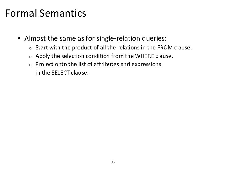
Formal Semantics • Almost the same as for single-relation queries: Start with the product of all the relations in the FROM clause. o Apply the selection condition from the WHERE clause. o Project onto the list of attributes and expressions in the SELECT clause. o 35

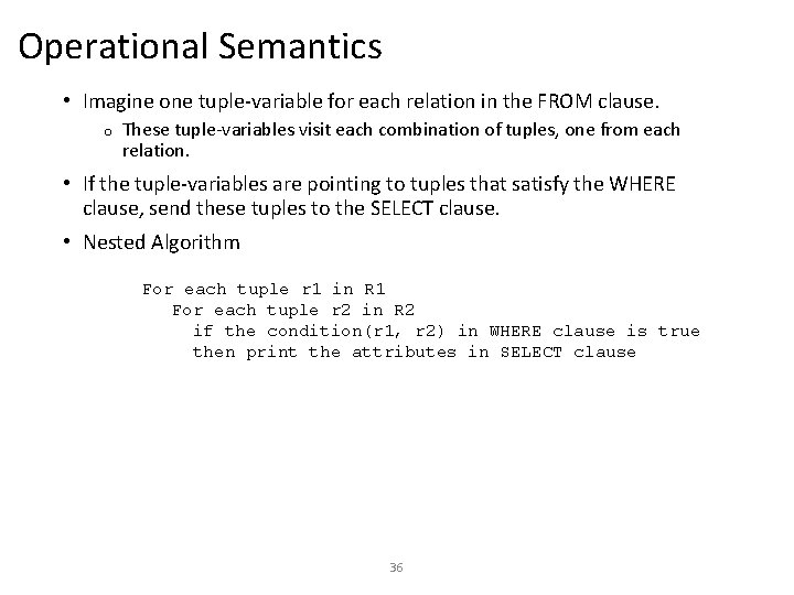
Operational Semantics • Imagine one tuple-variable for each relation in the FROM clause. o These tuple-variables visit each combination of tuples, one from each relation. • If the tuple-variables are pointing to tuples that satisfy the WHERE clause, send these tuples to the SELECT clause. • Nested Algorithm For each tuple r 1 in R 1 For each tuple r 2 in R 2 if the condition(r 1, r 2) in WHERE clause is true then print the attributes in SELECT clause 36

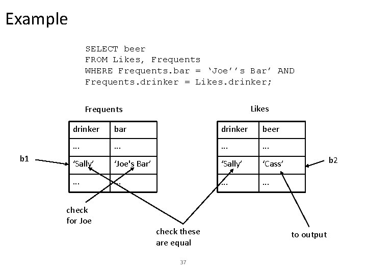
Example SELECT beer FROM Likes, Frequents WHERE Frequents. bar = ‘Joe’’s Bar’ AND Frequents. drinker = Likes. drinker; Likes Frequents b 1 drinker bar drinker beer . . . ‘Sally’ ‘Joe's Bar’ ‘Sally’ ‘Cass’ . . . check for Joe check these are equal 37 b 2 to output

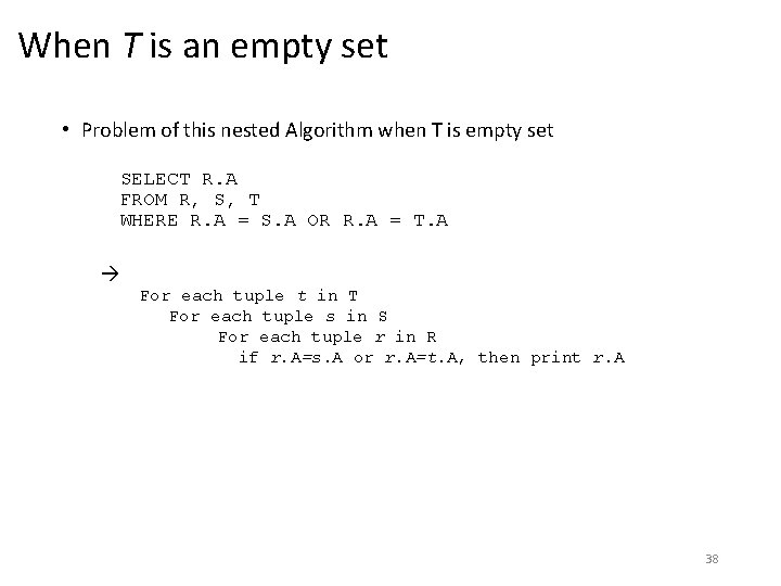
When T is an empty set • Problem of this nested Algorithm when T is empty set SELECT R. A FROM R, S, T WHERE R. A = S. A OR R. A = T. A For each tuple t in T For each tuple s in S For each tuple r in R if r. A=s. A or r. A=t. A, then print r. A 38

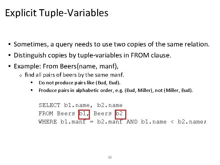
Explicit Tuple-Variables • Sometimes, a query needs to use two copies of the same relation. • Distinguish copies by tuple-variables in FROM clause. • Example: From Beers(name, manf), o find all pairs of beers by the same manf. § § Do not produce pairs like (Bud, Bud). Produce pairs in alphabetic order, e. g. (Bud, Miller), not (Miller, Bud). SELECT b 1. name, b 2. name FROM Beers b 1, Beers b 2 WHERE b 1. manf = b 2. manf AND b 1. name < b 2. name; 39

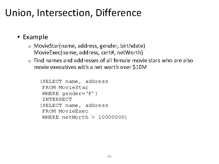
Union, Intersection, Difference • Example Movie. Star(name, address, gender, birthdate) Movie. Exec(name, address, cert#, net. Worth) o Find names and addresses of all female movie stars who are also movie executives with a net worth over $10 M o (SELECT name, address FROM Movie. Star WHERE gender=‘F’) INTERSECT (SELECT name, address FROM Movie. Exec WHERE net. Worth > 10000000) 40

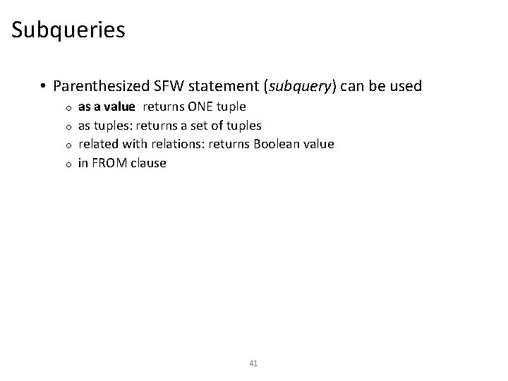
Subqueries • Parenthesized SFW statement (subquery) can be used as a value: returns ONE tuple o as tuples: returns a set of tuples o related with relations: returns Boolean value o in FROM clause o 41

Subqueries That Return One Tuple • If a subquery is guaranteed to produce one tuple, then the subquery can be used as a value (=, <, >, . . . ). Usually, the tuple has one component. o Also typically, a single tuple is guaranteed by “keyness” of attributes. o A run-time error occurs if there is no tuple or more than one tuple. o 42

Example • • From Sells(bar, beer, price), find the bars that serve Miller for the same price Joe charges for Miller. Two queries would surely work: 1. 2. Find the price Joe charges for Miller. Find the bars that serve Miller at that price. 43

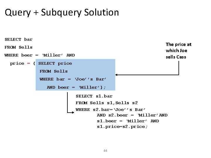
Query + Subquery Solution SELECT bar The price at which Joe sells Cass FROM Sells WHERE beer = ‘Miller’ AND price = ( SELECT price FROM Sells WHERE bar = ‘Joe’’s Bar’ AND beer = ‘Miller’); SELECT s 1. bar FROM Sells s 1, Sells s 2 WHERE s 2. bar=‘Joe’’s Bar’ AND s 2. beer = ‘Miller’AND s 1. beer = ‘Miller’ AND s 1. price=s 2. price; 44

Subqueries That Return More than one Tuple • If a subquery may produce more than one tuple, then the subquery can be used as a set of values o Set operator are used: IN and NOT IN operators o • IN operator <tuple> IN <relation> is true if and only if the tuple is a member of the relation. o <tuple> NOT IN <relation> means the opposite. o IN-expressions can appear in WHERE clauses. o The <relation> is often a subquery. o 45

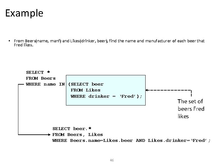
Example • From Beers(name, manf) and Likes(drinker, beer), find the name and manufacturer of each beer that Fred likes. SELECT * FROM Beers WHERE name IN (SELECT beer FROM Likes WHERE drinker = ‘Fred’); The set of beers Fred likes SELECT beer. * FROM Beers, Likes WHERE Beers. name=Likes. beer AND Likes. drinker=‘Fred’; 46

The Exists Operator • EXISTS( <relation> ) is true if and only if the <relation> is not empty. • Being a boolean-valued operator, EXISTS can appear in WHERE clauses. • Example: From Beers(name, manf), o find those beers that are the unique beer by their manufacturer. o 47

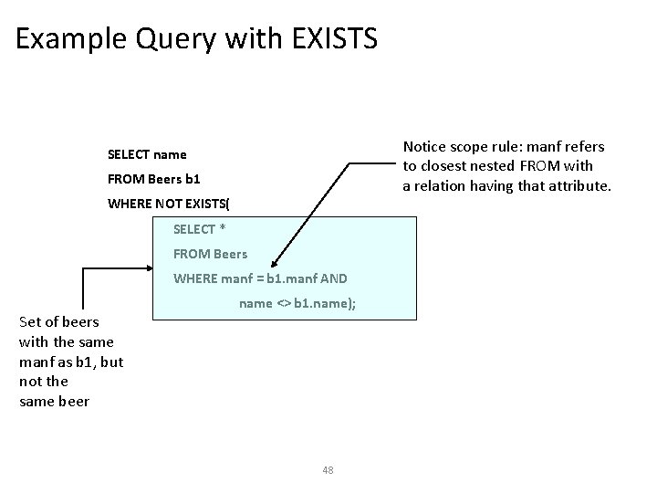
Example Query with EXISTS Notice scope rule: manf refers to closest nested FROM with a relation having that attribute. SELECT name FROM Beers b 1 WHERE NOT EXISTS( SELECT * FROM Beers WHERE manf = b 1. manf AND Set of beers with the same manf as b 1, but not the same beer name <> b 1. name); 48

The Operator ANY • x = ANY( <relation> ) is a Boolean condition meaning that x equals at least one tuple in the relation. • Similarly, = can be replaced by any of the comparison operators. • Example: x >= ANY( <relation> ) means x is not smaller than all tuples in the relation. o Note tuples must have one component only. 49

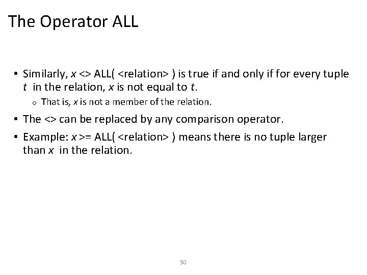
The Operator ALL • Similarly, x <> ALL( <relation> ) is true if and only if for every tuple t in the relation, x is not equal to t. o That is, x is not a member of the relation. • The <> can be replaced by any comparison operator. • Example: x >= ALL( <relation> ) means there is no tuple larger than x in the relation. 50

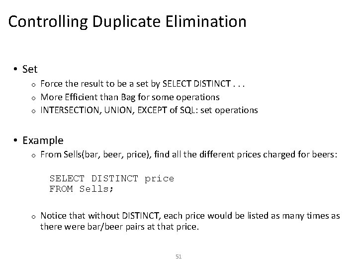
Controlling Duplicate Elimination • Set Force the result to be a set by SELECT DISTINCT. . . o More Efficient than Bag for some operations o INTERSECTION, UNION, EXCEPT of SQL: set operations o • Example o From Sells(bar, beer, price), find all the different prices charged for beers: SELECT DISTINCT price FROM Sells; o Notice that without DISTINCT, each price would be listed as many times as there were bar/beer pairs at that price. 51

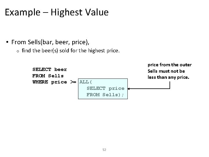
Example – Highest Value • From Sells(bar, beer, price), o find the beer(s) sold for the highest price. SELECT beer FROM Sells WHERE price >= ALL( SELECT price FROM Sells); 52 price from the outer Sells must not be less than any price.

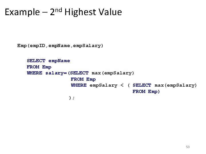
Example – 2 nd Highest Value Emp(emp. ID, emp. Name, emp. Salary) SELECT emp. Name FROM Emp WHERE salary=(SELECT max(emp. Salary) FROM Emp WHERE emp. Salary < ( SELECT max(emp. Salary) FROM Emp) ); 53

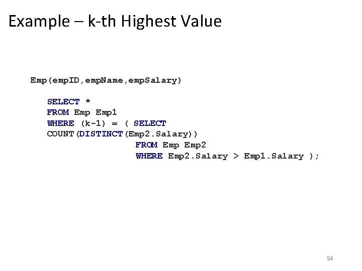
Example – k-th Highest Value Emp(emp. ID, emp. Name, emp. Salary) SELECT * FROM Emp 1 WHERE (k-1) = ( SELECT COUNT(DISTINCT(Emp 2. Salary)) FROM Emp 2 WHERE Emp 2. Salary > Emp 1. Salary ); 54

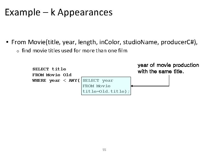
Example – k Appearances • From Movie(title, year, length, in. Color, studio. Name, producer. C#), o find movie titles used for more than one film SELECT title FROM Movie Old WHERE year < ANY( SELECT year FROM Movie title=Old. title); 55 year of movie production with the same title.

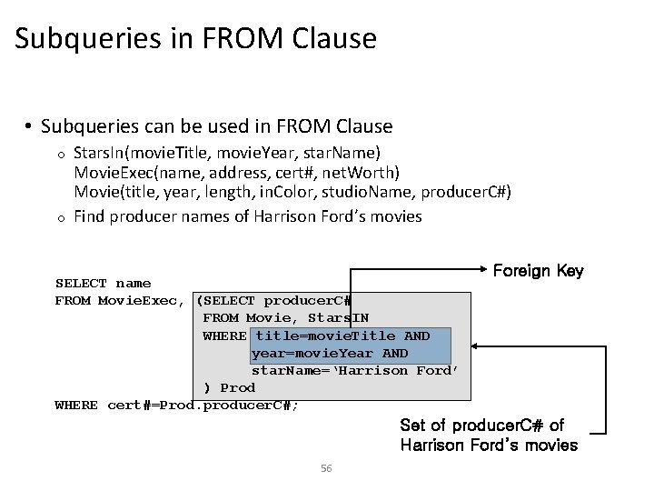
Subqueries in FROM Clause • Subqueries can be used in FROM Clause Stars. In(movie. Title, movie. Year, star. Name) Movie. Exec(name, address, cert#, net. Worth) Movie(title, year, length, in. Color, studio. Name, producer. C#) o Find producer names of Harrison Ford’s movies o SELECT name FROM Movie. Exec, (SELECT producer. C# FROM Movie, Stars. IN WHERE title=movie. Title AND year=movie. Year AND star. Name=‘Harrison Ford’ ) Prod WHERE cert#=Prod. producer. C#; Foreign Key Set of producer. C# of Harrison Ford’s movies 56

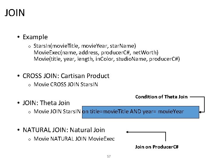
JOIN • Example o Stars. In(movie. Title, movie. Year, star. Name) Movie. Exec(name, address, producer. C#, net. Worth) Movie(title, year, length, in. Color, studio. Name, producer. C#) • CROSS JOIN: Cartisan Product o Movie CROSS JOIN Stars. IN Condition of Theta Join • JOIN: Theta Join o Movie JOIN Stars. IN on title=movie. Title AND year= movie. Year • NATURAL JOIN: Natural Join o Movie NATURAL JOIN Movie. Exec Join on Producer. C# 57

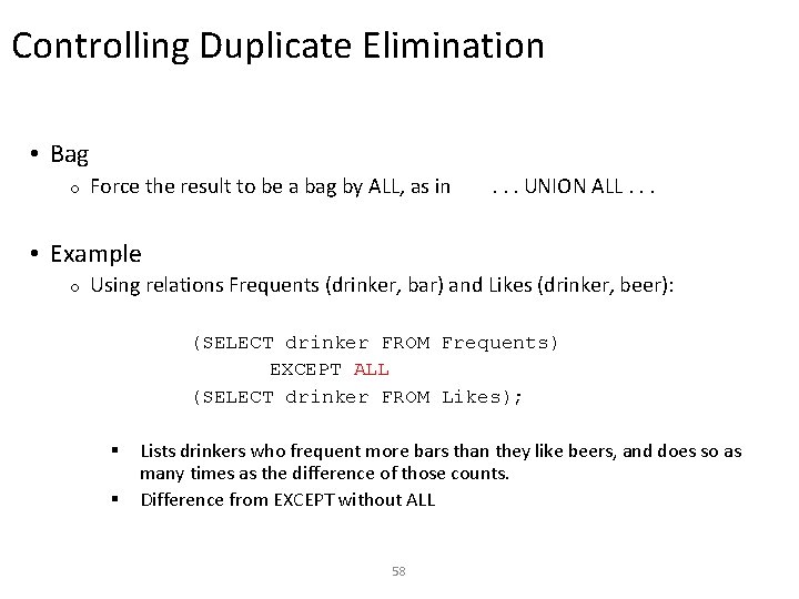
Controlling Duplicate Elimination • Bag o Force the result to be a bag by ALL, as in . . . UNION ALL. . . • Example o Using relations Frequents (drinker, bar) and Likes (drinker, beer): (SELECT drinker FROM Frequents) EXCEPT ALL (SELECT drinker FROM Likes); § § Lists drinkers who frequent more bars than they like beers, and does so as many times as the difference of those counts. Difference from EXCEPT without ALL 58

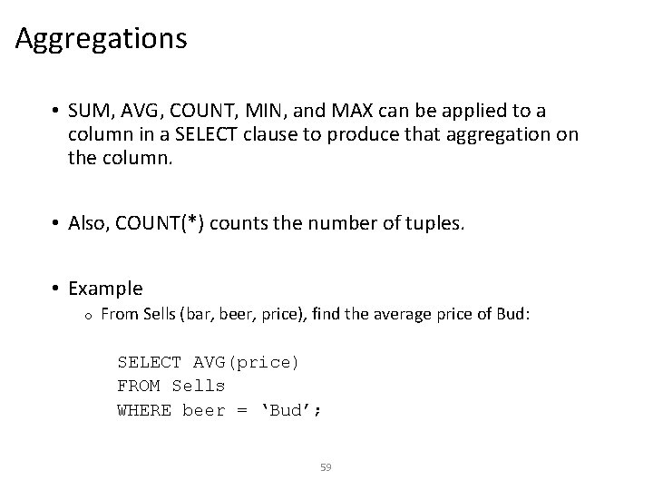
Aggregations • SUM, AVG, COUNT, MIN, and MAX can be applied to a column in a SELECT clause to produce that aggregation on the column. • Also, COUNT(*) counts the number of tuples. • Example o From Sells (bar, beer, price), find the average price of Bud: SELECT AVG(price) FROM Sells WHERE beer = ‘Bud’; 59

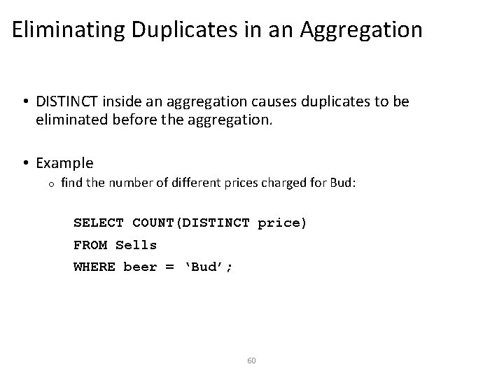
Eliminating Duplicates in an Aggregation • DISTINCT inside an aggregation causes duplicates to be eliminated before the aggregation. • Example o find the number of different prices charged for Bud: SELECT COUNT(DISTINCT price) FROM Sells WHERE beer = ‘Bud’; 60

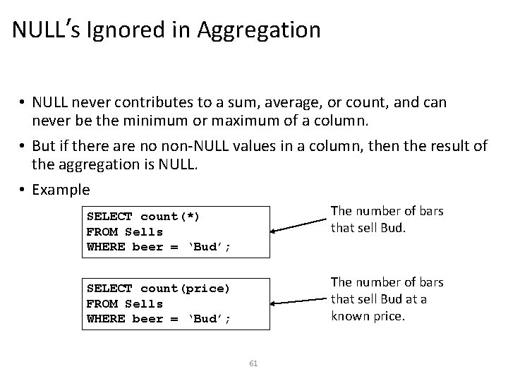
NULL’s Ignored in Aggregation • NULL never contributes to a sum, average, or count, and can never be the minimum or maximum of a column. • But if there are no non-NULL values in a column, then the result of the aggregation is NULL. • Example The number of bars that sell Bud. SELECT count(*) FROM Sells WHERE beer = ‘Bud’; The number of bars that sell Bud at a known price. SELECT count(price) FROM Sells WHERE beer = ‘Bud’; 61

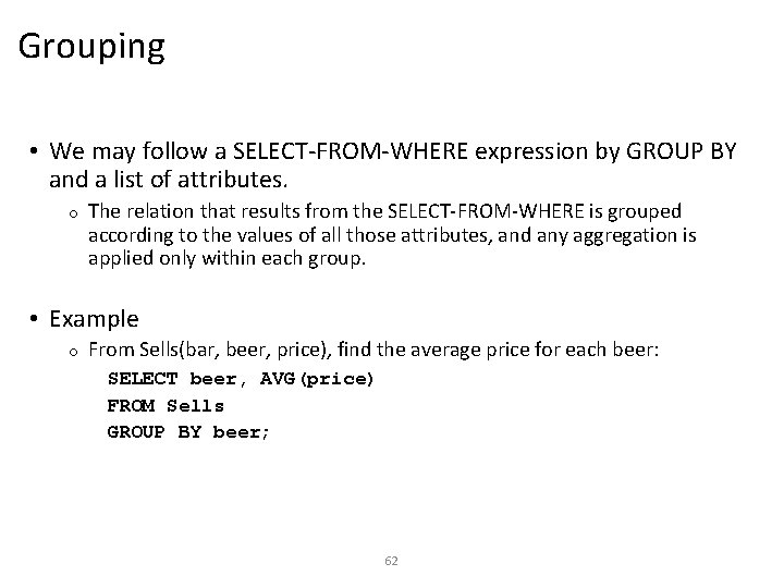
Grouping • We may follow a SELECT-FROM-WHERE expression by GROUP BY and a list of attributes. o The relation that results from the SELECT-FROM-WHERE is grouped according to the values of all those attributes, and any aggregation is applied only within each group. • Example o From Sells(bar, beer, price), find the average price for each beer: SELECT beer, AVG(price) FROM Sells GROUP BY beer; 62

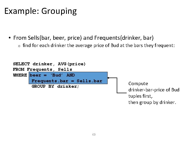
Example: Grouping • From Sells(bar, beer, price) and Frequents(drinker, bar) o find for each drinker the average price of Bud at the bars they frequent: SELECT drinker, AVG(price) FROM Frequents, Sells WHERE beer = ‘Bud’ AND Frequents. bar = Sells. bar GROUP BY drinker; 63 Compute drinker-bar-price of Bud tuples first, then group by drinker.

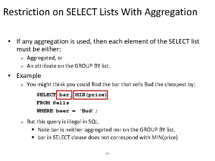
Restriction on SELECT Lists With Aggregation • If any aggregation is used, then each element of the SELECT list must be either: Aggregated, or o An attribute on the GROUP BY list. o • Example o You might think you could find the bar that sells Bud the cheapest by: SELECT bar, MIN(price) FROM Sells WHERE beer = ‘Bud’; o But this query is illegal in SQL. § Note bar is neither aggregated nor on the GROUP BY list. § bar in SELECT clause does not correspond with MIN(price) 64

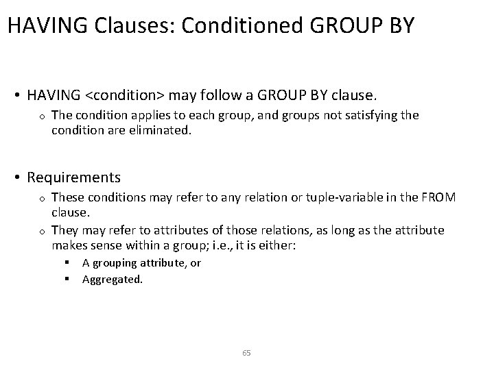
HAVING Clauses: Conditioned GROUP BY • HAVING <condition> may follow a GROUP BY clause. o The condition applies to each group, and groups not satisfying the condition are eliminated. • Requirements These conditions may refer to any relation or tuple-variable in the FROM clause. o They may refer to attributes of those relations, as long as the attribute makes sense within a group; i. e. , it is either: o § § A grouping attribute, or Aggregated. 65

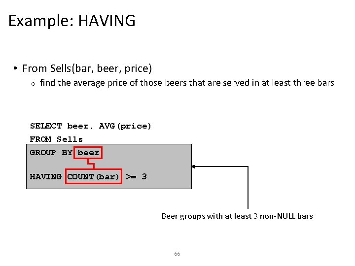
Example: HAVING • From Sells(bar, beer, price) o find the average price of those beers that are served in at least three bars SELECT beer, AVG(price) FROM Sells GROUP BY beer HAVING COUNT(bar) >= 3 Beer groups with at least 3 non-NULL bars 66

Database Modifications • A modification command does not return a result as a query does, but it changes the database in some way. • There are three kinds of modifications: Insert a tuple or tuples. o Delete a tuple or tuples. o Update the value(s) of an existing tuple or tuples. o 67

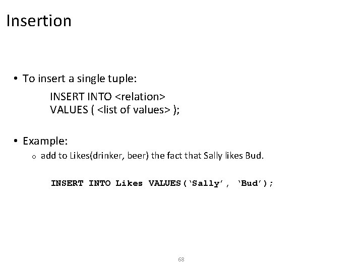
Insertion • To insert a single tuple: INSERT INTO <relation> VALUES ( <list of values> ); • Example: o add to Likes(drinker, beer) the fact that Sally likes Bud. INSERT INTO Likes VALUES(‘Sally’, ‘Bud’); 68

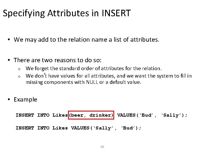
Specifying Attributes in INSERT • We may add to the relation name a list of attributes. • There are two reasons to do so: We forget the standard order of attributes for the relation. o We don’t have values for all attributes, and we want the system to fill in missing components with NULL or a default value. o • Example INSERT INTO Likes(beer, drinker) VALUES(‘Bud’, ‘Sally’); INSERT INTO Likes VALUES(‘Sally’, ‘Bud’); 69

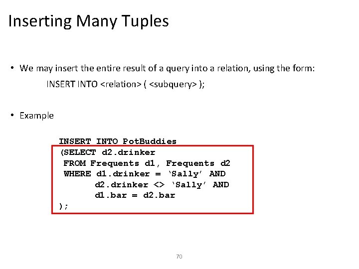
Inserting Many Tuples • We may insert the entire result of a query into a relation, using the form: INSERT INTO <relation> ( <subquery> ); • Example INSERT INTO Pot. Buddies (SELECT d 2. drinker FROM Frequents d 1, Frequents d 2 WHERE d 1. drinker = ‘Sally’ AND d 2. drinker <> ‘Sally’ AND d 1. bar = d 2. bar ); 70

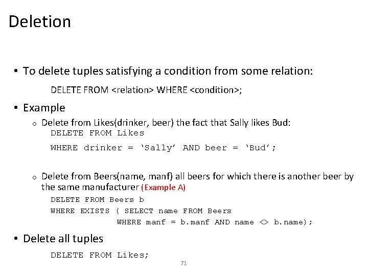
Deletion • To delete tuples satisfying a condition from some relation: DELETE FROM <relation> WHERE <condition>; • Example o Delete from Likes(drinker, beer) the fact that Sally likes Bud: DELETE FROM Likes WHERE drinker = ‘Sally’ AND beer = ‘Bud’; o Delete from Beers(name, manf) all beers for which there is another beer by the same manufacturer (Example A) DELETE FROM Beers b WHERE EXISTS ( SELECT name FROM Beers WHERE manf = b. manf AND name <> b. name); • Delete all tuples DELETE FROM Likes; 71

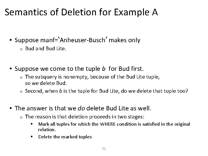
Semantics of Deletion for Example A • Suppose manf=‘Anheuser-Busch’ makes only o Bud and Bud Lite. • Suppose we come to the tuple b for Bud first. The subquery is nonempty, because of the Bud Lite tuple, so we delete Bud. o Second, when b is the tuple for Bud Lite, do we delete that tuple too? o • The answer is that we do delete Bud Lite as well. o The reason is that deletion proceeds in two stages: § § Mark all tuples for which the WHERE condition is satisfied in the original relation. Delete the marked tuples 72

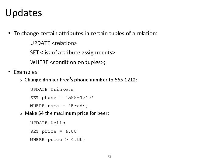
Updates • To change certain attributes in certain tuples of a relation: UPDATE <relation> SET <list of attribute assignments> WHERE <condition on tuples>; • Examples o Change drinker Fred’s phone number to 555 -1212: UPDATE Drinkers SET phone = ‘ 555 -1212’ WHERE name = ‘Fred’; o Make $4 the maximum price for beer: UPDATE Sells SET price = 4. 00 WHERE price > 4. 00; 73

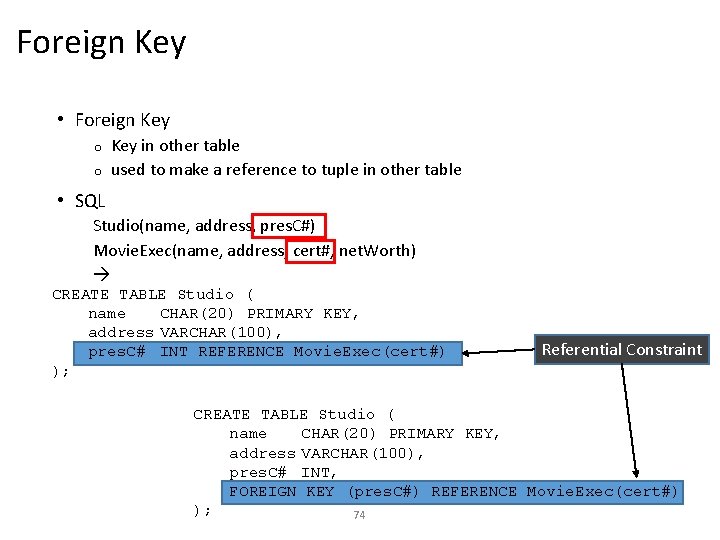
Foreign Key • Foreign Key in other table o used to make a reference to tuple in other table o • SQL Studio(name, address, pres. C#) Movie. Exec(name, address, cert#, net. Worth) CREATE TABLE Studio ( name CHAR(20) PRIMARY KEY, address VARCHAR(100), pres. C# INT REFERENCE Movie. Exec(cert#) ); Referential Constraint CREATE TABLE Studio ( name CHAR(20) PRIMARY KEY, address VARCHAR(100), pres. C# INT, FOREIGN KEY (pres. C#) REFERENCE Movie. Exec(cert#) ); 74

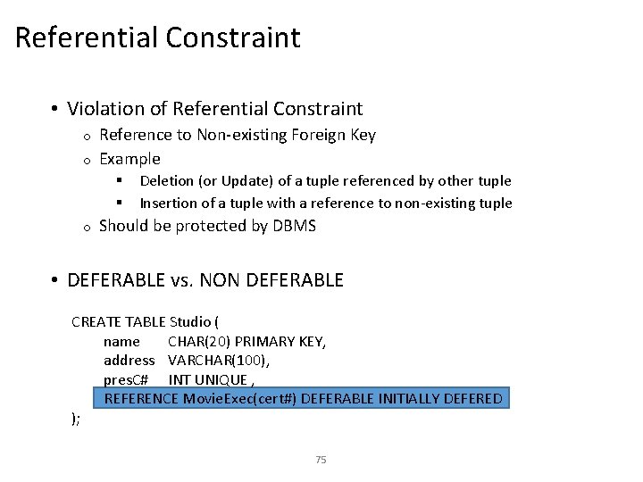
Referential Constraint • Violation of Referential Constraint Reference to Non-existing Foreign Key o Example o § § o Deletion (or Update) of a tuple referenced by other tuple Insertion of a tuple with a reference to non-existing tuple Should be protected by DBMS • DEFERABLE vs. NON DEFERABLE CREATE TABLE Studio ( name CHAR(20) PRIMARY KEY, address VARCHAR(100), pres. C# INT UNIQUE , REFERENCE Movie. Exec(cert#) DEFERABLE INITIALLY DEFERED ); 75

Index • Index Accelerating search speed o B+-tree, Hash etc. o • SQL CREATE INDEX Score. Index ON Student(score); CREATE INDEX Key. Index ON Movies(title, year); 76

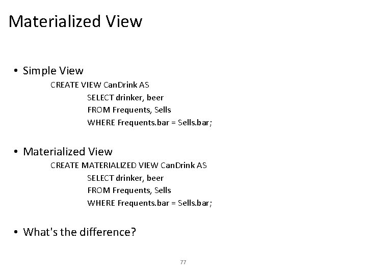
Materialized View • Simple View CREATE VIEW Can. Drink AS SELECT drinker, beer FROM Frequents, Sells WHERE Frequents. bar = Sells. bar; • Materialized View CREATE MATERIALIZED VIEW Can. Drink AS SELECT drinker, beer FROM Frequents, Sells WHERE Frequents. bar = Sells. bar; • What's the difference? 77