Review 21 06 2018 Study Design Study design

Review 21. 06. 2018

Study Design • Study design – Cohort – Case control – Cross sectional – Crossover • Epidemiologic concepts: – Bias – confounding

Statistics • Statistics – Descriptive statistics • Mean, median • Visual presentation (histogram, box plot) – Statistical tests • Univariate analysis – T test – Chi square – correlation • Multivariate analysis – Lineer regression – Logistic regression – Cox regression

The Concepts Should be Known • • • P value Confidence interval Power of the study Sample size Effect estimate – Relative risk – Odds ratio – Hazard ratio

Causal Relation between Independent and dependent variables B A C OUTCOME

Ratio, Proportion, Rate Is nominator included in denominator? NO YES Ratio Is the time included in denominator NO Proportion YES Rate

Summary: Objectives of the Course Program 1. Bias 2. Confounder Study Design Data collection Epidemiology 3. Chance Analysis: Statistical methods

RCT or Meta-analysis Non randomized but controlled Multicentric cohort or case control Expert opinion, descriptive, case series

Study Designs Does investigator decide for exposure? YES NO Experimental (interventional) Observational (non interventional) Randomization? Comparison Group YES RCT NO Non-randomized Controlled YES Analytical NO Descriptive

Study Designs exposure COHORT outcome exposure Case-control outcome Cross sectional Exposure Outcome

Schizophrenia CNS infection a No Schizophrenia b Study group Schizophrenia No infection c No Schizophrenia d

Retrospective Cohort Sonuç (outcome) exposed Sonuç yok Study group Sonuç yok Etkene maruz kalmayanlar (kontrol) Araştırmanın yönü zaman Onset of study

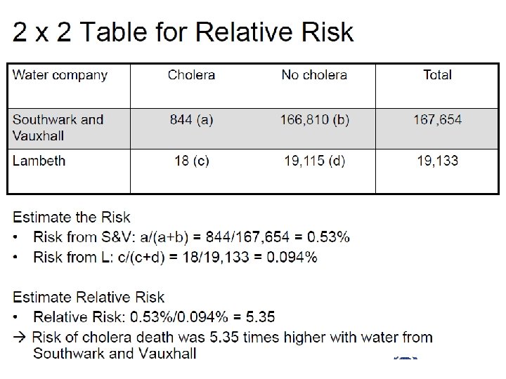
Relative Risk RR = Risk of exposed group a / (a + b) Risk of nonexposed group c / (c + d) = RR= incidence in exposed / incidence in nonexposed Outcome No outcome a b Nonexposed c d Exposed

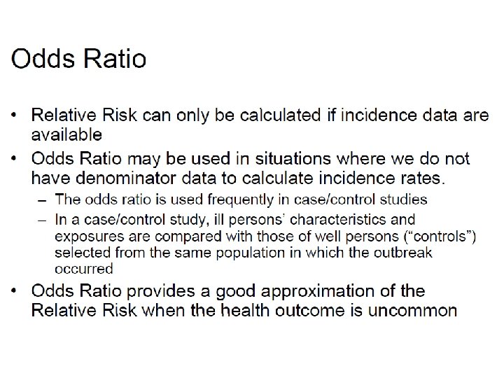
When OR is close to RR: Rare disease assumption a/ (a+b) RR= = c/ (c+d) a/b = c/d = OR ad bc Disease No disease exposed a b Nonexposed c d

Odds Ratio p = probability (or proportion) The lower bound is 0, and the upper bound is 1. Probability of success: Pr(y = 1) = p Probability of failure: Pr(y = 0) = 1 – p

What is the p of success or failure? Failure Success Total 1 -p p (1 - p) + p = 1 . 25 = 1 - p . 75 = p 1 = (1 - p) + p Odds = p/(1 -p) =. 75/ (1 -. 75) =. 75/. 25 = 3 Odds Ratio= p. A/(1 -p. A) p. B/(1 -p. B)

Relative Risk Heparin Plasebo Riskheparin= DVT 8 18 92 82 8/100 = 0. 08 Riskplasebo= 18/100 = 0. 18 Relative risk = Risk plasebo = Risk heparin 0. 18 0. 08 = 2. 25

Odds Ratio DVT Heparin Plasebo DVT 8 18 92 82 Oddsheparin= 8/92 = 0. 087 Oddsplasebo= 18/82 = 0. 22 Odds ratio = Odds plasebo = Odds heparin 0. 22 0. 087 = 2. 53

Comparing risks and odds Risk Odds 0. 05 or 5% 0. 053 0. 1 or 10% 0. 11 0. 2 or 20% 0. 25 0. 3 or 30% 0. 43 0. 4 or 40% 0. 67 0. 5 or 50% 1 0. 6 or 60% 1. 5 0. 7 or 70% 2. 3 0. 8 or 80% 4 0. 9 or 90% 9 0. 95 or 95% 19

The Confidence Interval for the Effect Size

The Confidence Interval for the Effect Size

Advantages of Cohort Studies cohort case-control Complete exposure information; Recall and selection bias Less bias for exposure Can examine temporal relation Not always Study multiple outcomes Only one outcome Incidence rates and RR OR Results easy to understand, straightforward More difficult interpretation

Disadvantages of Cohort Studies cohort case-control Inefficient for rare disease, unless the attributable risk percent is high Optimal for rare disease If prospective, extremely expensive and time consuming Cheaper and quick If retrospective, requires the availability of the records Validity of the results can be seriously affected by losses to follow-up

Case Control Study 26

Cross-over study design With outcome Experimental subjects Subjects meeting entry criteria Without outcome With outcome Controls Without outcome Onset of study With outcome Experimental subjects Intervention Without outcome Washout period Intervention Time 27

Randomized controlled trial design Experimental subjects With outcome Without outcome Subjects meeting entry criteria With outcome Controls Without outcome Time Onset of study Intervention 28

Objectives of the session • Data collection • Variables • Types of data • Central tendency measures • Central dispersion measures • Distribution of data

Presentation of Findings There are 3 main groups of tables in the results section of a scientific manuscript: 1. Demographic Characteristics of the Subjects 2. Univariate Analysis 3. Multivariate Analysis 30

Types of Numerical Data • Continuous: measurable quantities – Age – Cholesterol level 31

Types of Numerical Data • Categorical data – Nominal • Dichotomous or binary: male or female • Blood groups 32

Types of Numerical Data • Categorical data – Ordinal • The level of severity • Grading among cancer patients A 31 33

Variables String Nurse Physician Nurse Phycisian Lab tech Nurse Physician Lab tech numeric 1 1 2 3

Measures of Central Tendency • • mean median Mod Geometric mean

Non-normal (Asymmetrical) Distribution of Continous Variables 36

Measures of Dispersion Range Standard deviation Variance = SD 2 Percentile Interquartile range 37

Dispersion Measures Sedimentation values • Grup 1: 11, 12, 12, 13 • Grup 2: 4, 5, 6, 8, 19, 20, 21 sedim | Obs Mean Std. Dev. Min Max -------+--------------------------------grup 1 | 7 11. 85714. 6900656 11 13 sedim | Obs Mean Std. Dev. Min Max -------+--------------------------------grup 2 | 7 11. 85714 7. 733662 4 21

Standart Deviation X=mean n=number of subjects

Which one has bigger SD?

Tests for Normal Distribution • Visual methods – Histogram – Box plot • Statistical tests – Kolmogorov-Smirnov – Lilliefors – Shapiro wilk • Variation coefficient (SD/mean) – If SD/mean ≤%30, distribution ≈ normal

Histogram 42

Box plot

Standard Deviation vs Standard Error of the Mean (SOM) • The “standard error of the sample mean” depends on both the standard deviation and the sample size: SE = SD/ √(sample size) • The standard error decreases as the sample size increases, as the extent of chance variation is reduced. • By contrast the standard deviation will not tend to change as we increase the size of our sample. Altman DG. Standard deviations and standard errros. BMJ 2005; 331: 44903

Research Methodology: Epidemiology + Statistics • Epidemiology – John Snow, 1850 – Cohort boom, 1950 • Statistics; early 20 th century – K. Pearson – RA Fisher – J. Neyman The Lady Tasting Tea by David Salzburg

hypothesis testing 46

Effect Estimates • Relative Risk • Odds Ratio • Hazard Ratio

What is the role of chance? How do we understand the role of chance? • P value • Confidence intervals

What is p value ? The P value or calculated probability is the estimated probability of rejecting the null hypothesis (H 0) of a study question when that hypothesis is true.

The curve shown is represented as a probability density function. Data yielding a p-value of. 05 means there is only a 5% chance obtaining the observed (or more extreme) result if no real effect exists. "Common sense" tells us to judge our hypotheses based on how well they fit observed evidence. This is not what a p-value describes. Instead, it describes the likelihood of observing certain data given that the null hypothesis is true.

What is not P value? 1. 2. 3. 4. The probability of an event to occur Probability for true hypothesis Percentage for true hypothesis Proportion for true hypothesis

Testing Significance With a Confidence Interval One of the reasons confidence intervals are preferred over the p value, and why many journals discourage reporting a p value when the confidence interval is already reported, is that the confidence interval can be used for hypothesis testing. The method used is the chi-square test for a 2 2 table is identical to the z test for comparing two proportions

Confidence intervals instead of P value “For differences that are clinically important but not statistically significant, do not report a ‘trend toward significance. ’ Instead, report the observed difference and the (95%) confidence interval for the difference. When authors find a clinically important difference that is not statistically significant, they sometimes report that the difference shows a ‘trend’ (it cannot), it could just as easily move ‘away from’ the alpha level as ‘toward’ it. ” Lang and Secic. How to Report Statistics in Medicine, 2006

The Confidence Interval for the Effect Size

Confidence Intervals When an estimate is presented as a single value, such as an odds ratio, we refer to it as a point estimate of the population odds ratio. When we compute a confidence interval, we form a interval estimate of the value. A confidence interval is called an interval estimate, which is a interval (lower bound , upper bound) that we can be confident covers, or straddles, the true population effect with some level of confidence. The interpretation of a 95% confidence interval for the odds ratio is (van Belle et al, 2004, p. 86): The probability is 0. 95, or 95%, that the interval (lower bound , upper bound) straddles the population odds ratio.

Inclusion of “ 1” or not 57/54

Hypothesis Testing Test result True situation Ho correct H 1 correct Ho accept OK Type II error Ho reject Type I error Power 58

Exposure - Outcome Test result True situation Drug equal to placebo Drug better/worse than placebo Drug equal to placebo Ho Drug better/worse than placebo H 1 OK Type II error β Type I error α OK 59

Calculation of the Sample Size 1. Type I error (α), usually <0. 05, false positivity 2. Type II error (β), usually <0. 2, false negativity 3. Power (=1 -β): The probability of the detection of a real difference as statistically significant If β=0. 20, the power 80% ü The difference between 2 groups can be detected by the probability of 80% 4. Minimum expected difference 5. Estimated measurement variability 60

Univariate Analysis: Comparison of 2 Groups Variable Continuous Categorical Is distribution Normal? Non-parametric tests 61

Univariate Analysis: Comparison of 2 Groups Continuous variable Symmetric (Normal) distribution Asymmetric distribution Student t test Mann-Whitney-U test 62 Willcoxon test

Chi Squared Test A chi-squared test, also referred to as chi-square test or test, is any statistical hypothesis test in which the sampling distribution of the test statistic is a chi-squared distribution when the null hypothesis is true, or any in which this is asymptotically true, meaning that the sampling distribution (if the null hypothesis is true) can be made to approximate a chi-squared distribution as closely as desired by making the sample size large enough.

Statistical tests NULL hypothesis: Mean. GREEN = Mean. BLUE ALTERNATIVE hypothesis: Mean. GREEN ≠ Mean. BLUE

Types of Statistical Tests (a few examples) Univariate Non. Parametric - No specified population parameter Parametric - Population parameter specified Multivariate Chi-square test Extensions of univariate - Of independence tests (see left) - Goodness of fit Mann-Whitney U Wilcoxon signed rank test Kruskal-Wallis 1 -way ANOVA z – test t – tests 1 -factor (1 -way) ANOVA Regression 2 -factor ANOVA Regression techniques (multiple regression)

Univariate Analysis: Correlation Systolic blood pressure r = 0. 70 60 70 80 90 100 Body weight 66

Multivariate analyses Regression Dependent variable (outcome) Linear Continuous Logistic Dichotomous Cox Dichotomous Poisson Dichotomous

Confounder Variable A Outcome Variable B

Confounder Acinetobacter infection fatality Severity index APACHE score

The control of the confounders 1. Randomization 2. Stratification 3. Adjustment by multivariate analysis

Confounder OC MI Smoking

An example Outcome : Deep Vein Thrombosis Independent variables : Heparin, gender, Coronary Heart Disease, aspirin use Y= a+b 1 x 1+ b 2 x 2 + b 3 x 3 + b 4 x 4 DVT=a+b 1(heparin)+ b 2(female) + b 3(CAD)+ b 4(aspirin) 0. 5 1. 5 3 0. 6

Logistic regression Number of obs LR chi 2(4) Prob > chi 2 Pseudo R 2 Log likelihood = -6. 2444702 = = 10 0. 97 0. 9141 0. 0722 --------------------------------------DVT | Odds Ratio Std. Err. z P>|z| [95% Conf Interval] -------+-------------------------------Heparin |. 50. 023 -2. 81 0. 003. 15. 72 Kadin | 1. 48 1. 08 0. 01 0. 504. 095 23. 17 KAH | 3. 06. 03 2. 36 0. 009 1. 34 12. 37 aspirin | 0. 58 0. 08 0. 31 0. 622. 46 1. 03 -------------------------------------- OR p-değeri 95% CI Heparin use 0. 5 0. 003 0. 15 -0. 72 Female 1. 48 0. 504 0. 095 -23. 17 CHD 3. 06 0. 009 1. 34 -12. 37 Aspirin use 0. 58 0. 622 0. 46 -1. 03

Study Protocol Title Background: 1 -2 paragraph What is the knowledge on this field? Why do we need this study? Knowledge gaps Hypothesis: 1 sentence The shortest is the best Method Study population: campus, hospital, etc. Sample size calculation Survey, laboratory, Impact of the study References Institutional Review Board

Timeline for Study Projects October 2015 Proposal October. November 2015 Applications Permissions IRB November December January February Data Collection April 2016 March 2016 Data Analysis Presentation & Report

Oct Proposal IRB Permissions Data collection Analysis Presentation Report Nov Dec Jan Feb March April