Retrospective Cohort Study 1 Review Retrospective Cohort Study

Retrospective Cohort Study 1

Review- Retrospective Cohort Study Retrospective cohort study: • Investigator has access to exposure data on a group of people. • The study sample is divided into exposed and non-exposed groups. • Both the exposures and outcomes of interest have already occurred (hence “retrospective”). • The disease experience of exposed and nonexposed groups is compared (e. g. risk ratio or rate ratio). 2

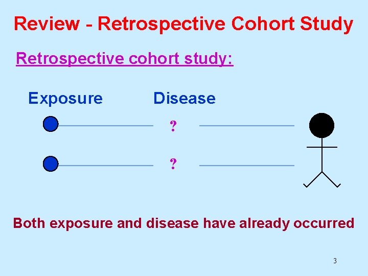
Review - Retrospective Cohort Study Retrospective cohort study: Exposure Disease ? ? Both exposure and disease have already occurred 3

Retrospective Cohort Studies (Also called “historical” studies) 4

Design Features Strengths: • Can study the effects of exposures that no longer occur (e. g. discontinued medical treatments. ) • Quicker and less costly than prospective cohort studies. • Particularly efficient for study of rare exposures, especially occupational and “natural history” exposures. 5

Design Features Strengths (cont. ): • Particularly efficient for studying diseases with long “latency” periods. • Can examine multiple effects of single exposure. • Can yield information on multiple exposures. • May allow direct measurement of incidence of disease in exposed and non-exposed groups (hence, calculation of relative risk). 6

Design Features Limitations: • Not useful for study of emerging, new exposures. • Reliance on existing records or subject recall may be less accurate and complete than data collected prospectively (e. g. records were not recorded for the hypothesis of interest). • Information on potential confounding factors are often unavailable from existing records. 7

IMPORTANT CONCEPTS IN COHORT STUDIES • Rates Versus Risks • Calculating Person Time • Estimating the Empirical Induction Period • Estimating Effect of Relevant Exposure 8

Rates Versus Risks • In some instances, it is more desirable to calculate and compare incidence rates, rather than incidence proportions (risks). -- Recall, cumulative incidence provides an estimate of the probability (risk) that an individual will develop a disease during a specified period of time. -- Whereas, an incidence rate centers on how fast new cases are occurring in a population. 9

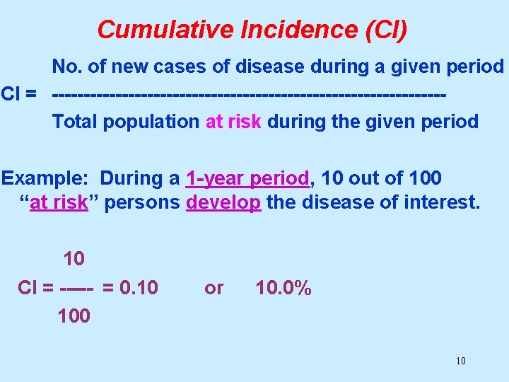
Cumulative Incidence (CI) No. of new cases of disease during a given period CI = -------------------------------Total population at risk during the given period Example: During a 1 -year period, 10 out of 100 “at risk” persons develop the disease of interest. 10 CI = ----- = 0. 10 100 or 10. 0% 10

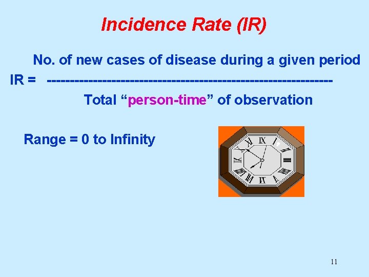
Incidence Rate (IR) No. of new cases of disease during a given period IR = -------------------------------Total “person-time” of observation Range = 0 to Infinity 11

Incidence Rate (IR) What is person time? When we observe a group of individuals for a period of time in order to ascertain the DEVELOPMENT of an event…. -The actual time each individual is observed will most likely vary. 12

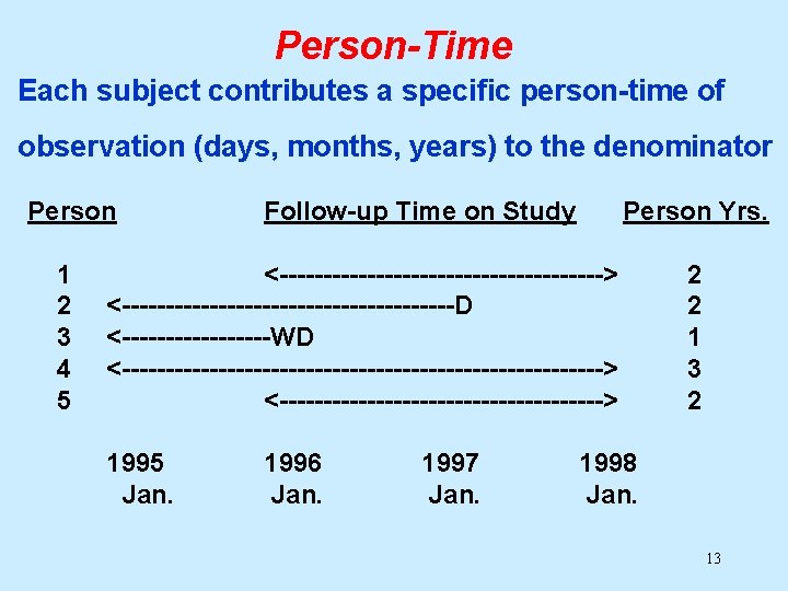
Person-Time Each subject contributes a specific person-time of observation (days, months, years) to the denominator Person 1 2 3 4 5 Follow-up Time on Study Person Yrs. <-------------------> <-------------------D <---------WD <----------------------------> <-------------------> 1995 Jan. 1996 Jan. 1997 Jan. 2 2 1 3 2 1998 Jan. 13

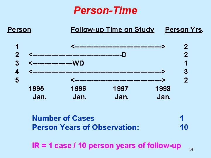
Person-Time Person 1 2 3 4 5 Follow-up Time on Study Person Yrs. <-------------------> <-------------------D <---------WD <----------------------------> <-------------------> 1995 1996 1997 1998 Jan. Number of Cases Person Years of Observation: 2 2 1 3 2 1 10 IR = 1 case / 10 person years of follow-up 14

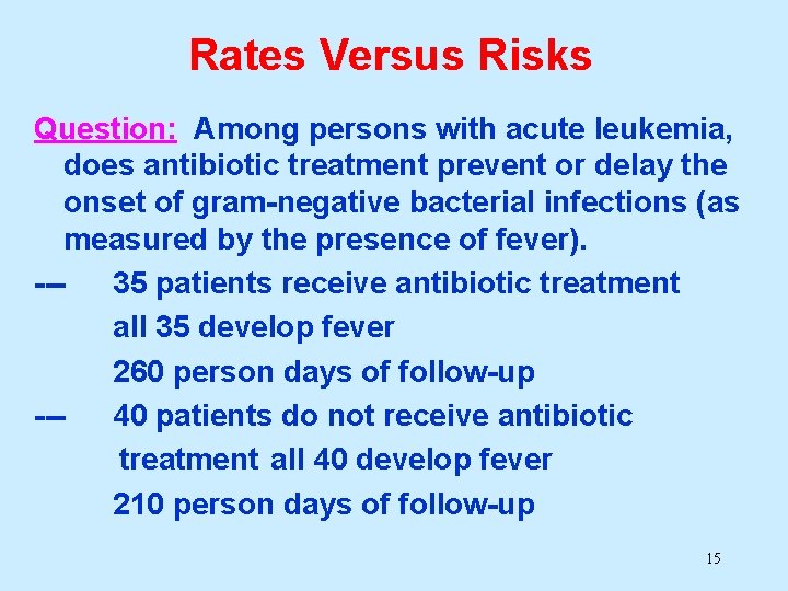
Rates Versus Risks Question: Among persons with acute leukemia, does antibiotic treatment prevent or delay the onset of gram-negative bacterial infections (as measured by the presence of fever). --35 patients receive antibiotic treatment all 35 develop fever 260 person days of follow-up --40 patients do not receive antibiotic treatment all 40 develop fever 210 person days of follow-up 15

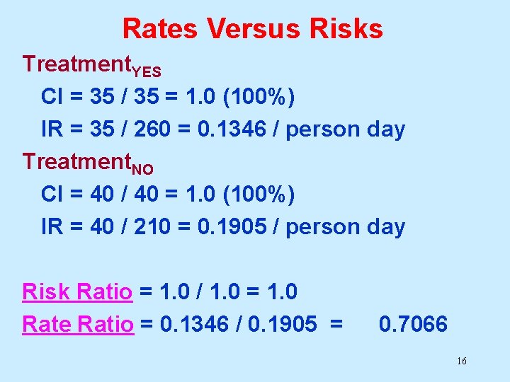
Rates Versus Risks Treatment. YES CI = 35 / 35 = 1. 0 (100%) IR = 35 / 260 = 0. 1346 / person day Treatment. NO CI = 40 / 40 = 1. 0 (100%) IR = 40 / 210 = 0. 1905 / person day Risk Ratio = 1. 0 / 1. 0 = 1. 0 Rate Ratio = 0. 1346 / 0. 1905 = 0. 7066 16

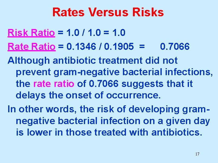
Rates Versus Risk Ratio = 1. 0 / 1. 0 = 1. 0 Rate Ratio = 0. 1346 / 0. 1905 = 0. 7066 Although antibiotic treatment did not prevent gram-negative bacterial infections, the ratio of 0. 7066 suggests that it delays the onset of occurrence. In other words, the risk of developing gramnegative bacterial infection on a given day is lower in those treated with antibiotics. 17

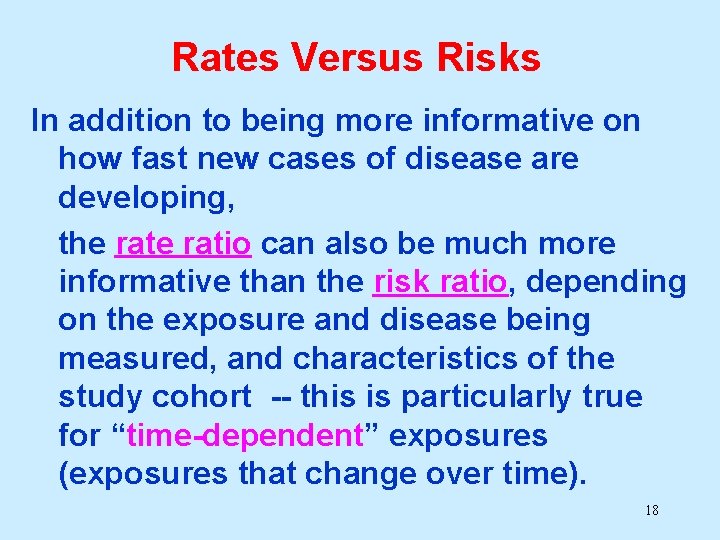
Rates Versus Risks In addition to being more informative on how fast new cases of disease are developing, the ratio can also be much more informative than the risk ratio, depending on the exposure and disease being measured, and characteristics of the study cohort -- this is particularly true for “time-dependent” exposures (exposures that change over time). 18

Definitions “Open” or “Dynamic” Population: Population in which person-time experience can accrue from a changing roster of individuals. “Fixed Cohort”: Exposure groups are defined at the start of follow-up with no movement of individuals between exposure groups (e. g. clinical trial). “Closed” Cohort or Population: Fixed cohort with no loss to follow-up. 19

Estimating Relevant Exposure When exposures are “dynamic, ” it is important take into account these changes as subjects are followed. Example: Suppose a cohort of industrial workers are continuously exposed to a hazardous agent over the course of their working career. We wish to compare the mortality experience of those with low, moderate, and high exposure to mortality in the general population (see handouts). 20

Estimating Relevant Exposure Whether implicit or explicit, and whether for cohort studies or case-control studies, it is important to consider the empirical induction period when estimating the effects of exposures. 21

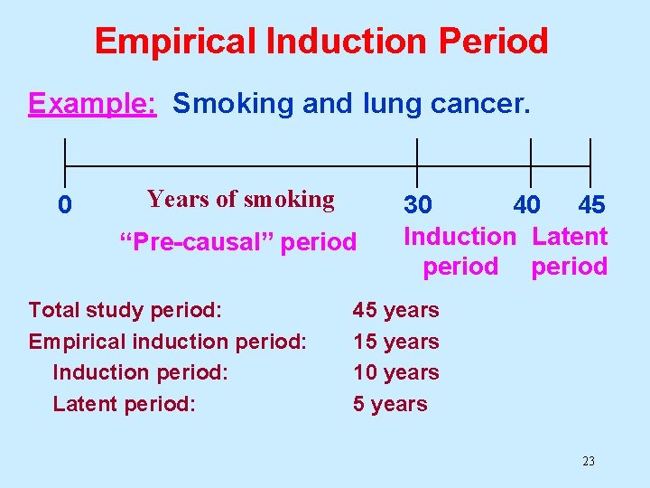
Empirical Induction Period The “empirical induction period” includes the time from causal action of the exposure to disease detection. This consists of 2 parts: • Induction period: Period of time from causal action to disease initiation (triggering). • Latent period: Time interval between disease occurrence and detection. 22

Empirical Induction Period Example: Smoking and lung cancer. 0 Years of smoking “Pre-causal” period Total study period: Empirical induction period: Induction period: Latent period: 30 40 45 Induction Latent period 45 years 10 years 5 years 23

Empirical Induction Period For many exposure/disease associations, the empirical induction period is unknown. The latent period can be reduced by improved methods of disease detection. Slow-growing cancers may appear to have long induction periods with respect to some causes because they have long latent periods. 24

Estimating Relevant Exposure Depending on the empirical induction period, it is often inappropriate to uniformly assign persons as exposed or non-exposed. Instead, persons can contribute person time to both exposed and non-exposed denominators. In other words, the time at risk of disease may vary depending on levels of the accumulation and intensity of exposure. 25

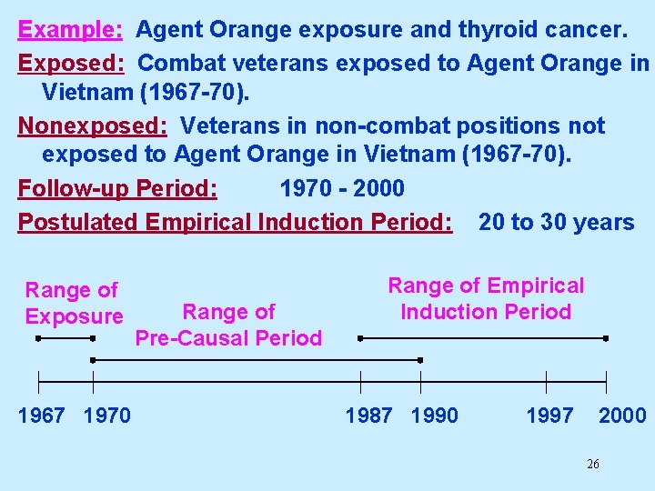
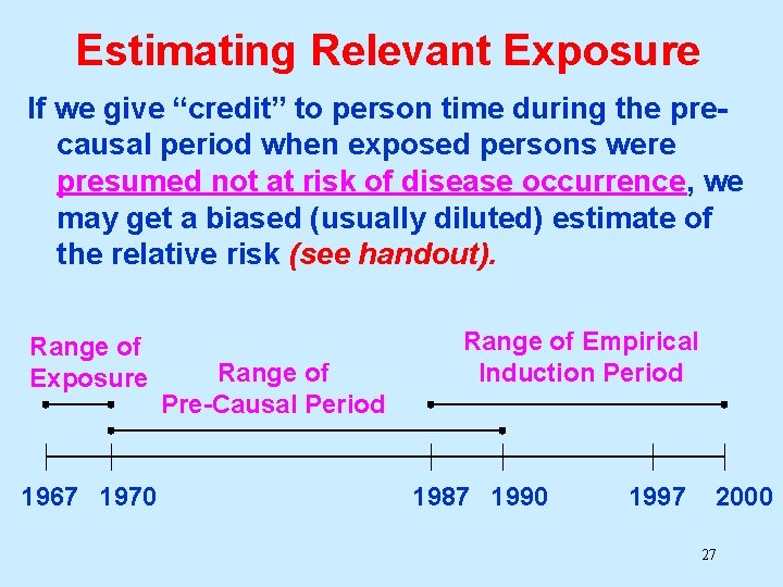
Example: Agent Orange exposure and thyroid cancer. Exposed: Combat veterans exposed to Agent Orange in Vietnam (1967 -70). Nonexposed: Veterans in non-combat positions not exposed to Agent Orange in Vietnam (1967 -70). Follow-up Period: 1970 - 2000 Postulated Empirical Induction Period: 20 to 30 years Range of Exposure 1967 1970 Range of Pre-Causal Period Range of Empirical Induction Period 1987 1990 1997 2000 26

Estimating Relevant Exposure If we give “credit” to person time during the precausal period when exposed persons were presumed not at risk of disease occurrence, we may get a biased (usually diluted) estimate of the relative risk (see handout). Range of Exposure 1967 1970 Range of Pre-Causal Period Range of Empirical Induction Period 1987 1990 1997 2000 27

Estimating Relevant Exposure An important issue is what happens to the time experienced by exposed subjects that does not meet the definition of time at risk of exposure effects (the empirical induction period). The non-relevant follow-up time can be: 1. Assigned to the denominator of the unexposed rate. 2. Excluded from the study. 28

Estimating Relevant Exposure Advantages of assigning the non-relevant follow-up time to the denominator of the unexposed rate: • Greater precision in estimating the rate among the unexposed. • Greater comparability between the exposed and non-exposed on characteristics such as age and time period of follow-up. 29

Estimating Relevant Exposure Disadvantage of assigning the non-relevant follow-up time to the denominator of the unexposed rate: • If the empirical induction period is underestimated, truly “exposed” cases will be added to the rate of the non-exposed – this will tend to make the exposed and unexposed rates more similar than they really are. 30

Estimating Relevant Exposure Disadvantage of excluding the non-relevant follow-up time to the denominator of the unexposed rate: • The number of truly unexposed cases may be too small to produce a stable comparison. 31

Estimating Relevant Exposure Since the empirical induction period is often unknown, how do we know if it is appropriate? • The empirical induction period can be “lagged” with separate analyses conducted using each period -- e. g. 10 to 20 years 15 to 25 years 20 to 30 years 25 to 35 years 30 to 40 years 35 to 45 years 32

Estimating Relevant Exposure If multiple empirical induction periods are analyzed: • One can select the largest risk estimate, with the tenuous assumption that it is not the largest simply due to statistical variability (chance). • The data should be inspected to see whether a consistent pattern of effects emerges that reflect the empirical induction period. 33

Timing of Outcome Events To accurately estimate person time of follow-up, it is important to determine the time of the event as precisely as possible. Example: Defining the onset of time for disorders such as multiple sclerosis and atherosclerosis can be ambiguous. 34

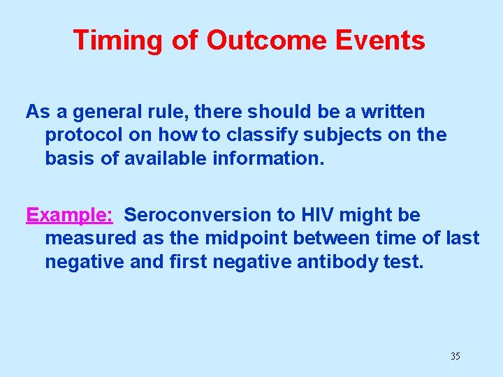
Timing of Outcome Events As a general rule, there should be a written protocol on how to classify subjects on the basis of available information. Example: Seroconversion to HIV might be measured as the midpoint between time of last negative and first negative antibody test. 35