Reintroduction to Factorial Designs 5 terms necessary to

Reintroduction to Factorial Designs • 5 terms necessary to understand factorial designs • 5 patterns of factorial results for a 2 x 2 factorial designs • Descriptive & misleading main effects • Research Hypotheses for factorial designs • Other ways of thinking about inteactions • Factorial designs in programmatic research

Other Ways of Thinking About Interactions • Ways of Describing Interactions other than “Simple Effects” • Interactions as “other kinds of” cell mean difference patterns • Interactions as “non-additive combinations” of IV effects • augmenting vs. interfering interactions • Describing “interactions” vs. “data patterns” • isolating the interaction effect

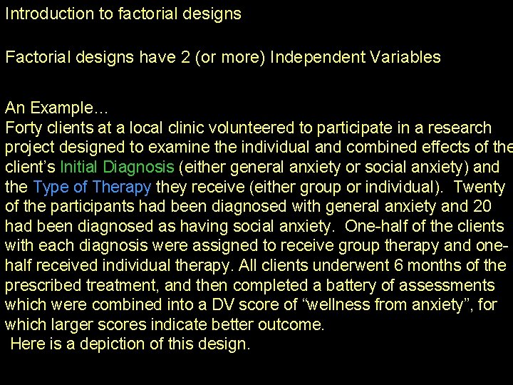
Introduction to factorial designs Factorial designs have 2 (or more) Independent Variables An Example… Forty clients at a local clinic volunteered to participate in a research project designed to examine the individual and combined effects of the client’s Initial Diagnosis (either general anxiety or social anxiety) and the Type of Therapy they receive (either group or individual). Twenty of the participants had been diagnosed with general anxiety and 20 had been diagnosed as having social anxiety. One-half of the clients with each diagnosis were assigned to receive group therapy and onehalf received individual therapy. All clients underwent 6 months of the prescribed treatment, and then completed a battery of assessments which were combined into a DV score of “wellness from anxiety”, for which larger scores indicate better outcome. Here is a depiction of this design.

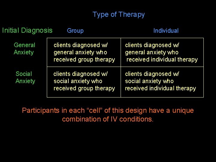
Type of Therapy Initial Diagnosis Group Individual General Anxiety clients diagnosed w/ general anxiety who received group therapy clients diagnosed w/ general anxiety who received individual therapy Social Anxiety clients diagnosed w/ social anxiety who received group therapy clients diagnosed w/ social anxiety who received individual therapy Participants in each “cell” of this design have a unique combination of IV conditions.

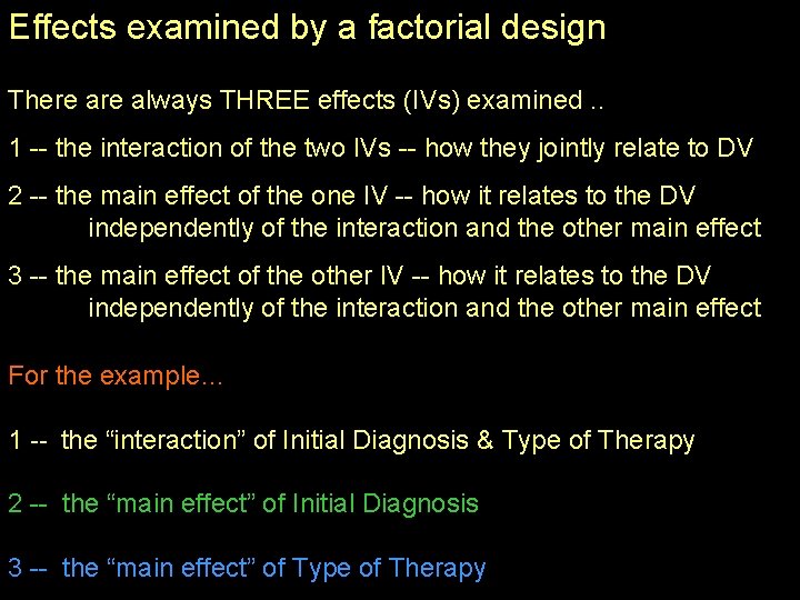
Effects examined by a factorial design There always THREE effects (IVs) examined. . 1 -- the interaction of the two IVs -- how they jointly relate to DV 2 -- the main effect of the one IV -- how it relates to the DV independently of the interaction and the other main effect 3 -- the main effect of the other IV -- how it relates to the DV independently of the interaction and the other main effect For the example… 1 -- the “interaction” of Initial Diagnosis & Type of Therapy 2 -- the “main effect” of Initial Diagnosis 3 -- the “main effect” of Type of Therapy

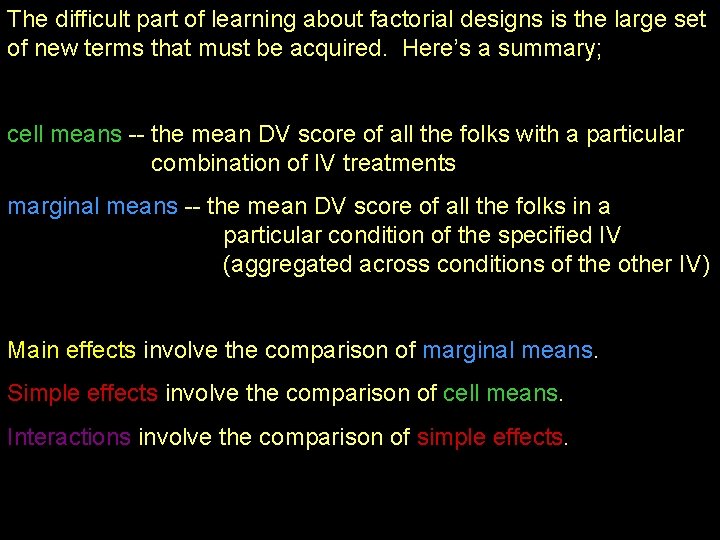
The difficult part of learning about factorial designs is the large set of new terms that must be acquired. Here’s a summary; cell means -- the mean DV score of all the folks with a particular combination of IV treatments marginal means -- the mean DV score of all the folks in a particular condition of the specified IV (aggregated across conditions of the other IV) Main effects involve the comparison of marginal means. Simple effects involve the comparison of cell means. Interactions involve the comparison of simple effects.

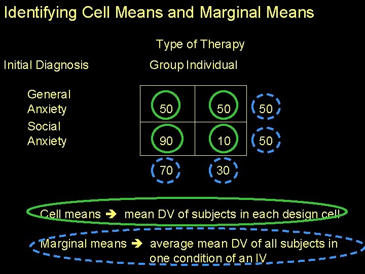
Identifying Cell Means and Marginal Means Type of Therapy Initial Diagnosis General Anxiety Social Anxiety Group Individual 50 50 50 90 10 50 70 30 Cell means mean DV of subjects in each design cell Marginal means average mean DV of all subjects in one condition of an IV

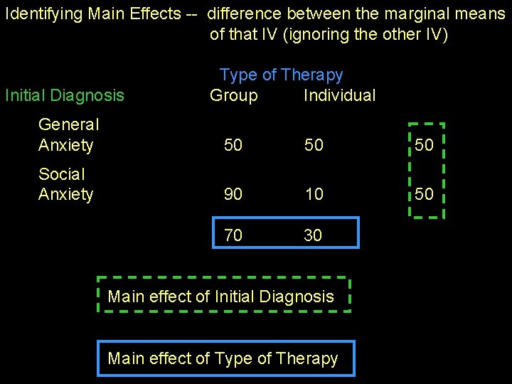
Identifying Main Effects -- difference between the marginal means of that IV (ignoring the other IV) Initial Diagnosis Type of Therapy Group Individual General Anxiety 50 50 50 Social Anxiety 90 10 50 70 30 Main effect of Initial Diagnosis Main effect of Type of Therapy

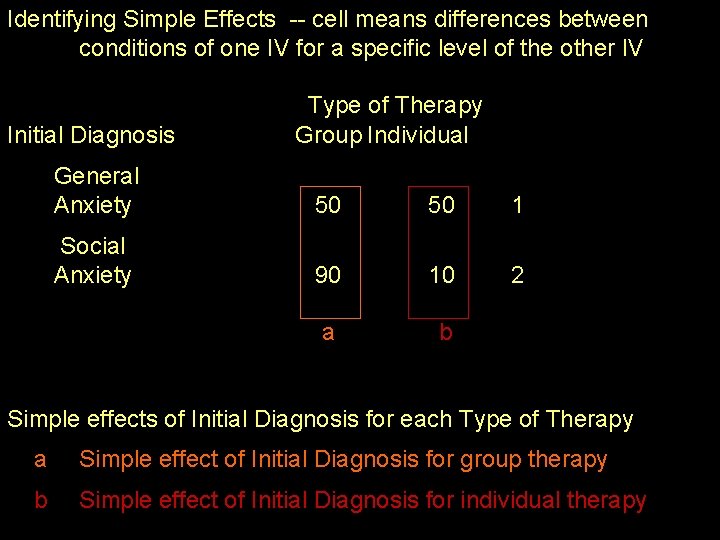
Identifying Simple Effects -- cell means differences between conditions of one IV for a specific level of the other IV Initial Diagnosis Type of Therapy Group Individual General Anxiety 50 50 1 Social Anxiety 90 10 2 a b Simple effects of Initial Diagnosis for each Type of Therapy a Simple effect of Initial Diagnosis for group therapy b Simple effect of Initial Diagnosis for individual therapy

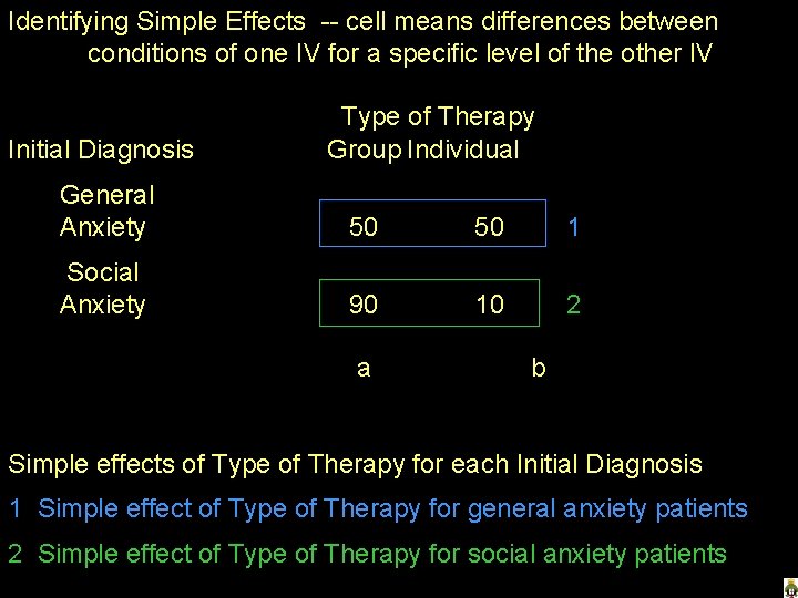
Identifying Simple Effects -- cell means differences between conditions of one IV for a specific level of the other IV Initial Diagnosis Type of Therapy Group Individual General Anxiety 50 50 1 Social Anxiety 90 10 2 a b Simple effects of Type of Therapy for each Initial Diagnosis 1 Simple effect of Type of Therapy for general anxiety patients 2 Simple effect of Type of Therapy for social anxiety patients

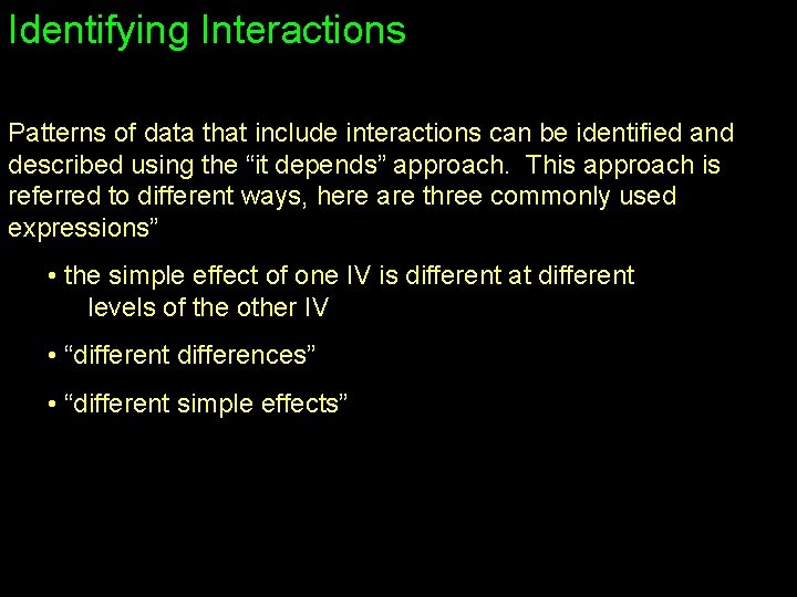
Identifying Interactions Patterns of data that include interactions can be identified and described using the “it depends” approach. This approach is referred to different ways, here are three commonly used expressions” • the simple effect of one IV is different at different levels of the other IV • “different differences” • “different simple effects”

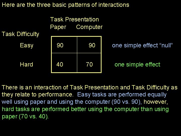
Here are three basic patterns of interactions Task Presentation Paper Computer Task Difficulty Easy 90 Hard 40 90 70 one simple effect “null” one simple effect There is an interaction of Task Presentation and Task Difficulty as they relate to performance. Easy tasks are performed equally well using paper and using the computer (90 vs. 90), however, hard tasks are performed better using the computer than using paper (70 vs. 40).

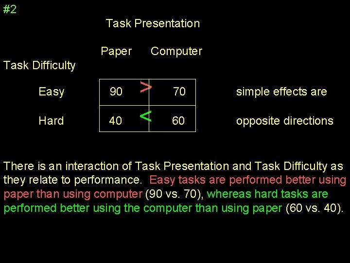
#2 Task Presentation Paper Computer Task Difficulty Easy 90 Hard 40 > < 70 simple effects are 60 opposite directions There is an interaction of Task Presentation and Task Difficulty as they relate to performance. Easy tasks are performed better using paper than using computer (90 vs. 70), whereas hard tasks are performed better using the computer than using paper (60 vs. 40).

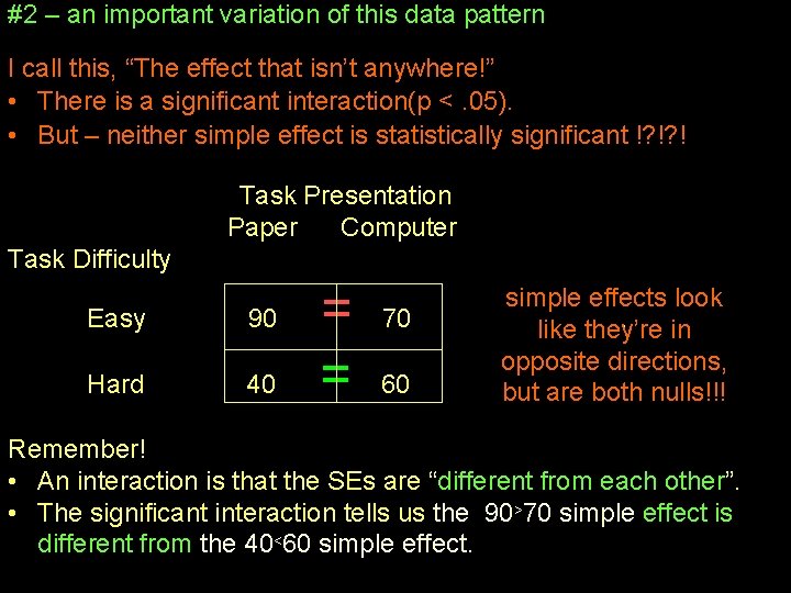
#2 – an important variation of this data pattern I call this, “The effect that isn’t anywhere!” • There is a significant interaction(p <. 05). • But – neither simple effect is statistically significant !? !? ! Task Presentation Paper Computer Task Difficulty Easy 90 Hard 40 = = 70 60 simple effects look. like they’re in opposite directions, but are both nulls!!! Remember! • An interaction is that the SEs are “different from each other”. • The significant interaction tells us the 90>70 simple effect is different from the 40<60 simple effect.

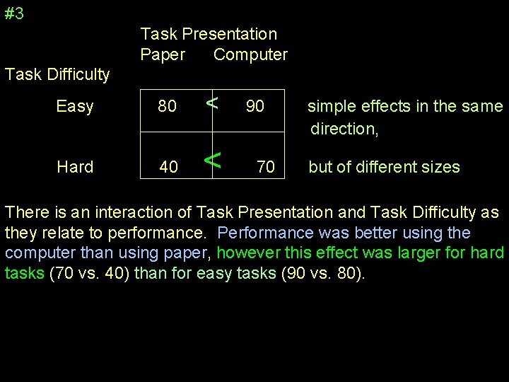
#3 Task Presentation Paper Computer Task Difficulty Easy 80 < Hard 40 < 90 70 simple effects in the same direction, but of different sizes There is an interaction of Task Presentation and Task Difficulty as they relate to performance. Performance was better using the computer than using paper, however this effect was larger for hard tasks (70 vs. 40) than for easy tasks (90 vs. 80).

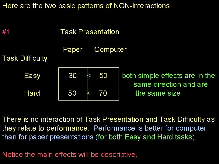
Here are the two basic patterns of NON-interactions #1 Task Presentation Paper Computer Task Difficulty Easy 30 < 50 Hard 50 < 70 both simple effects are in the same direction and are the same size There is no interaction of Task Presentation and Task Difficulty as they relate to performance. Performance is better for computer than for paper presentations (for both Easy and Hard tasks). Notice the main effects will be descriptive.

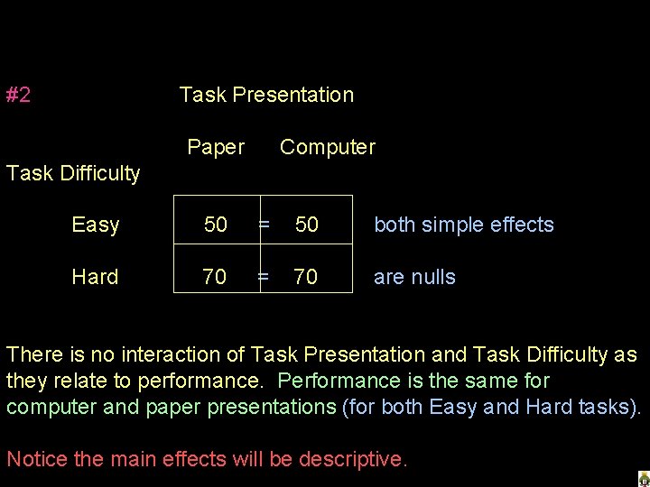
#2 Task Presentation Paper Computer Task Difficulty Easy 50 = 50 both simple effects Hard 70 = 70 are nulls There is no interaction of Task Presentation and Task Difficulty as they relate to performance. Performance is the same for computer and paper presentations (for both Easy and Hard tasks). Notice the main effects will be descriptive.

Identifying Main Effects Patterns of data that include main effects can be identified by looking at the differences among the marginal means for a specific IV (the main effect of each IV must be examined and described separately !!!) • When there is an interaction, each main effect (null or significant) must be carefully examined to determine if that main effect is • “descriptive” (unconditional, that is, descriptive for all levels of the other IV) or is • “potentially misleading (conditional, that is, descriptive for only some or none of the levels of the other IV) • You must determine whether the pattern of each main effect (direction of any difference between the marginal means) is equivalent to each of the corresponding simple effects of that variable at the various levels of the other I

Importance or Main Effects ? ? It is not uncommon to hear the advice to “ignore main effects if there is an interaction. ” My best guess is that this is based on the correct idea that the pattern of some interactions can render the pattern of one or both main effects to be potentially or completely misleading. However, it is also possible that there can be an interaction and that one or both of the main effects can be descriptive. Discerning whether main effects are descriptive or misleading is a critical step in the examination of data from a factorial design! You must ensure that the reader has a thorough understanding of the pattern of your data! You must give a complete accounting of each of the three effects involved in the factorial design, the interaction and each of the main effects!

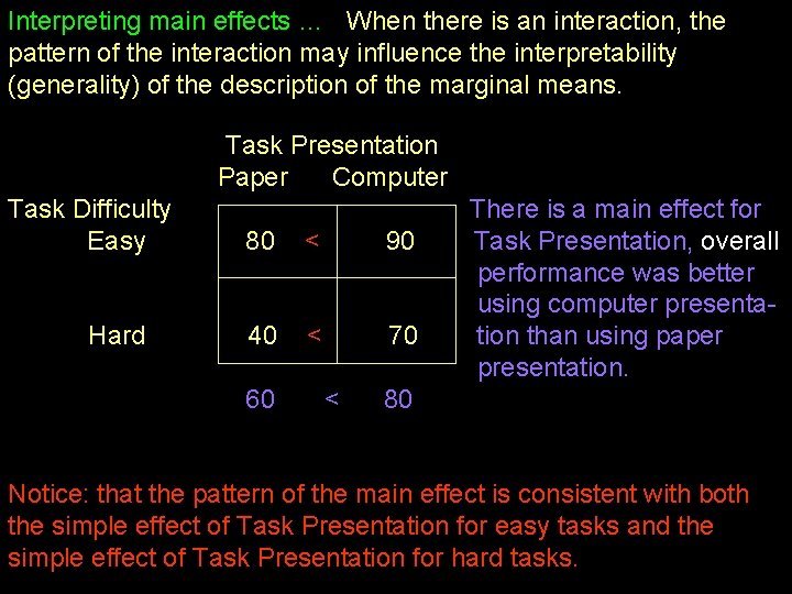
Interpreting main effects … When there is an interaction, the pattern of the interaction may influence the interpretability (generality) of the description of the marginal means. Task Presentation Paper Computer Task Difficulty Easy Hard 80 < 90 40 < 70 60 < There is a main effect for Task Presentation, overall performance was better using computer presentation than using paper presentation. 80 Notice: that the pattern of the main effect is consistent with both the simple effect of Task Presentation for easy tasks and the simple effect of Task Presentation for hard tasks.

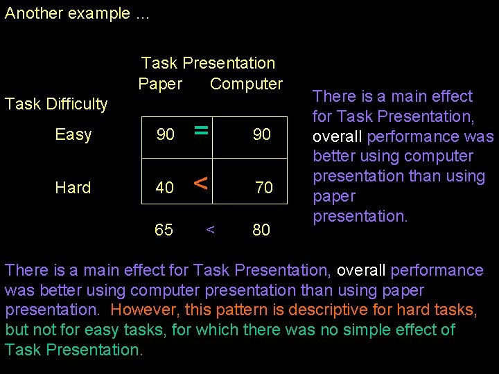
Another example … Task Presentation Paper Computer Task Difficulty Easy 90 = 90 Hard 40 < 70 65 < 80 There is a main effect for Task Presentation, overall performance was better using computer presentation than using paper presentation. However, this pattern is descriptive for hard tasks, but not for easy tasks, for which there was no simple effect of Task Presentation.

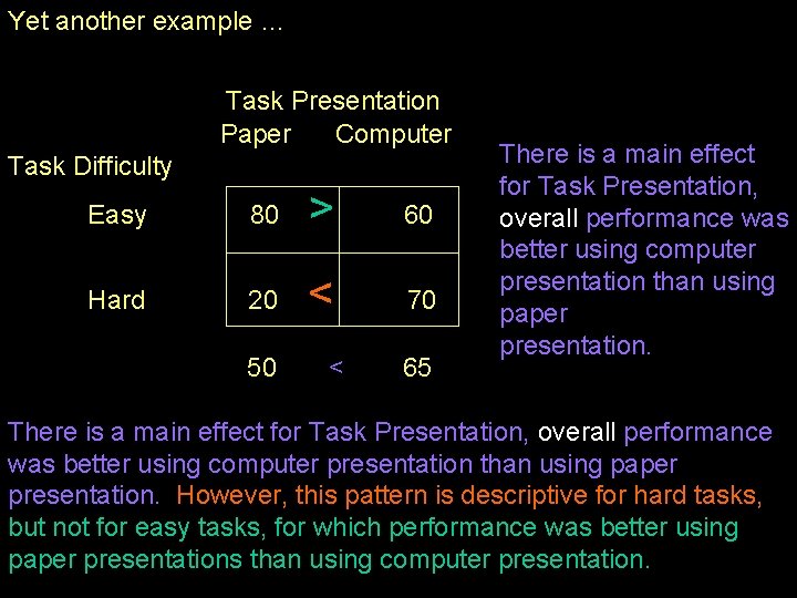
Yet another example … Task Presentation Paper Computer Task Difficulty Easy 80 > 60 Hard 20 < 70 50 < 65 There is a main effect for Task Presentation, overall performance was better using computer presentation than using paper presentation. However, this pattern is descriptive for hard tasks, but not for easy tasks, for which performance was better using paper presentations than using computer presentation.

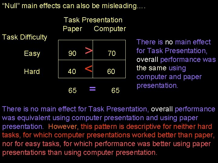
“Null” main effects can also be misleading…. Task Presentation Paper Computer Task Difficulty Easy 90 Hard 40 65 > < = 70 60 65 There is no main effect for Task Presentation, overall performance was the same using computer and paper presentation. There is no main effect for Task Presentation, overall performance was equivalent using computer presentation and using paper presentation. However, this pattern is descriptive for neither hard tasks, for which computer presentations worked better than paper, nor for easy tasks, for which performance was better using paper presentations than using computer presentation.

Related to this is the very important issue of whether or not the 2 -way interactions and main effects that are part of the 3 -way design “mean anything to us” ? ? ? It all goes back to “representation & inference” !!! Remember – the purpose of any design condition or value is to represent some population so we can infer that the difference between those conditions or values in the design represent differences between the populations we really care about! The “cells” in the 2 -way each represent a specific population and so, comparisons between them are comparisons between out target populations. But the means/values of all the main effects are “aggregates” – who do they represent? ? ?

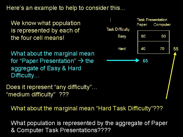
Here’s an example to help to consider this… We know what population is represented by each of the four cell means! What about the marginal mean for “Paper Presentation” the aggregate of Easy & Hard Difficulty… 55 65 Does it represent “any difficulty”… “medium difficulty” ? ? ? What about the marginal mean “Hard Task Difficulty”? ? ? What population is represented by the aggregate of Paper & Computer Task Presentations? ?

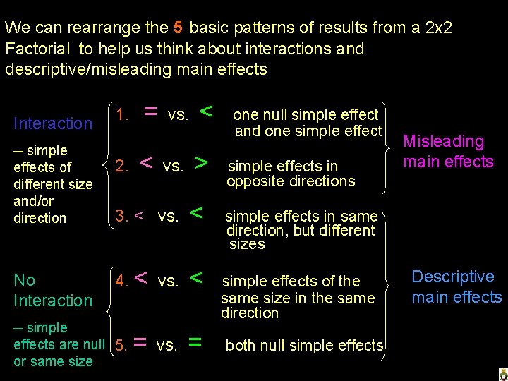
We can rearrange the 5 basic patterns of results from a 2 x 2 Factorial to help us think about interactions and descriptive/misleading main effects Interaction -- simple effects of different size and/or direction No Interaction 1. = < vs. > 3. < vs. < 4. < vs. < 2. -- simple effects are null 5. or same size < vs. = one null simple effect and one simple effects in opposite directions Misleading main effects simple effects in same direction, but different sizes simple effects of the same size in the same direction both null simple effects Descriptive main effects

RH: for Factorial Designs Research hypotheses for factorial designs may include • RH: for main effects • involve the effects of one IV, while ignoring the other IV • tested by comparing the appropriate marginal means • RH: for interactions • usually expressed as “different differences” -- differences between a set of simple effects • tested by comparing the results of the appropriate set of simple effects • That’s the hard part -- determining which set of simple effects gives the most direct test of the interaction RH:

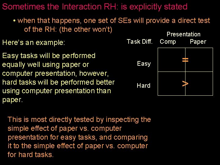
Sometimes the Interaction RH: is explicitly stated • when that happens, one set of SEs will provide a direct test of the RH: (the other won’t) Here’s an example: Easy tasks will be performed equally well using paper or computer presentation, however, hard tasks will be performed better using computer presentation than paper. Task Diff. Presentation Comp Paper Easy = Hard > This is most directly tested by inspecting the simple effect of paper vs. computer presentation for easy tasks, and comparing it to the simple effect of paper vs. computer for hard tasks.

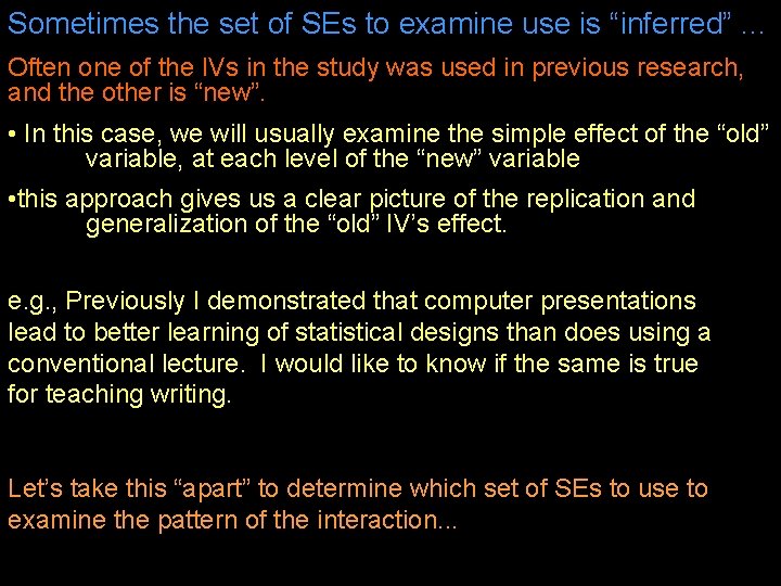
Sometimes the set of SEs to examine use is “inferred”. . . Often one of the IVs in the study was used in previous research, and the other is “new”. • In this case, we will usually examine the simple effect of the “old” variable, at each level of the “new” variable • this approach gives us a clear picture of the replication and generalization of the “old” IV’s effect. e. g. , Previously I demonstrated that computer presentations lead to better learning of statistical designs than does using a conventional lecture. I would like to know if the same is true for teaching writing. Let’s take this “apart” to determine which set of SEs to use to examine the pattern of the interaction. . .

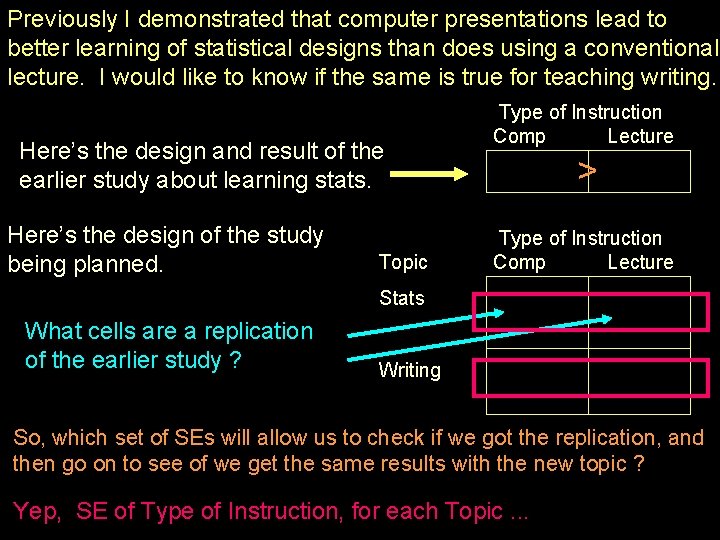
Previously I demonstrated that computer presentations lead to better learning of statistical designs than does using a conventional lecture. I would like to know if the same is true for teaching writing. Here’s the design and result of the earlier study about learning stats. Here’s the design of the study being planned. Topic Type of Instruction Comp Lecture > Type of Instruction Comp Lecture Stats What cells are a replication of the earlier study ? Writing So, which set of SEs will allow us to check if we got the replication, and then go on to see of we get the same results with the new topic ? Yep, SE of Type of Instruction, for each Topic. . .

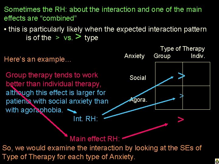
Sometimes the RH: about the interaction and one of the main effects are “combined” • this is particularly likely when the expected interaction pattern is of the > vs. > type Here’s an example… Group therapy tends to work better than individual therapy, although this effect is larger for patients with social anxiety than with agoraphobia. Int. RH: Anxiety Type of Therapy Group Indiv. Social > Agora. > > Main effect RH: So, we would examine the interaction by looking at the SEs of Type of Therapy for each type of Anxiety.

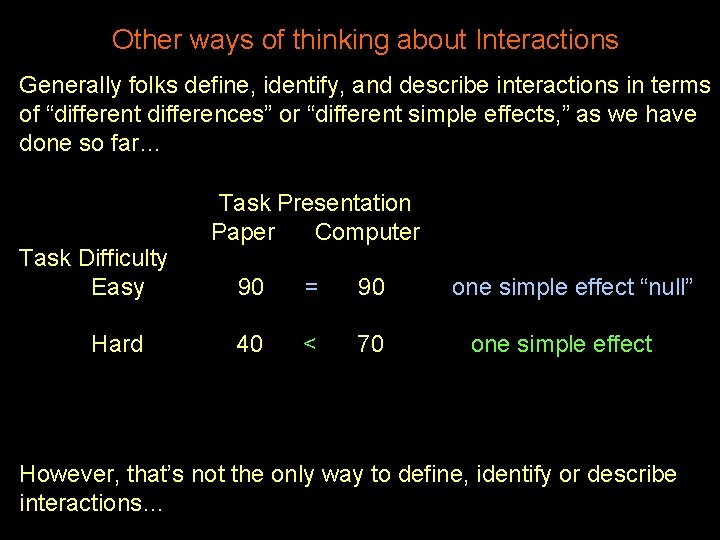
Other ways of thinking about Interactions Generally folks define, identify, and describe interactions in terms of “different differences” or “different simple effects, ” as we have done so far… Task Difficulty Easy Hard Task Presentation Paper Computer 90 = 90 40 < 70 one simple effect “null” one simple effect However, that’s not the only way to define, identify or describe interactions…

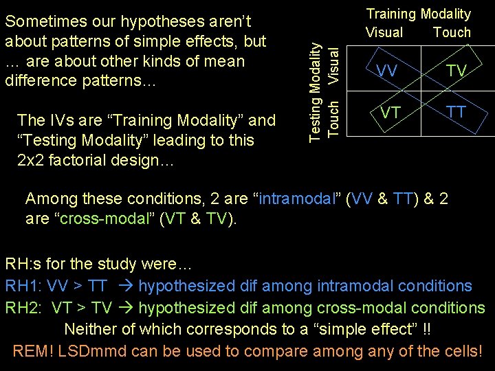
The IVs are “Training Modality” and “Testing Modality” leading to this 2 x 2 factorial design… Training Modality Visual Touch Testing Modality Touch Visual Sometimes our hypotheses aren’t about patterns of simple effects, but … are about other kinds of mean difference patterns… VV TV VT TT Among these conditions, 2 are “intramodal” (VV & TT) & 2 are “cross-modal” (VT & TV). RH: s for the study were… RH 1: VV > TT hypothesized dif among intramodal conditions RH 2: VT > TV hypothesized dif among cross-modal conditions Neither of which corresponds to a “simple effect” !! REM! LSDmmd can be used to compare among any of the cells!

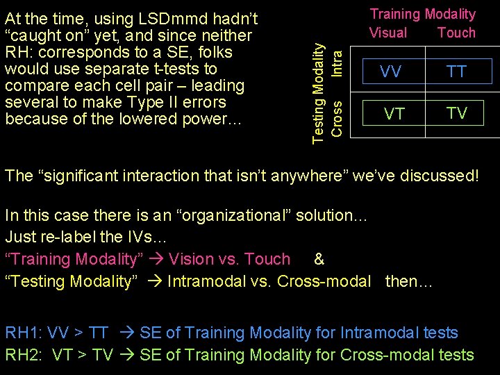
Training Modality Visual Touch Testing Modality Cross Intra At the time, using LSDmmd hadn’t “caught on” yet, and since neither RH: corresponds to a SE, folks would use separate t-tests to compare each cell pair – leading several to make Type II errors because of the lowered power… VV TT VT TV The “significant interaction that isn’t anywhere” we’ve discussed! In this case there is an “organizational” solution… Just re-label the IVs… “Training Modality” Vision vs. Touch & “Testing Modality” Intramodal vs. Cross-modal then… RH 1: VV > TT SE of Training Modality for Intramodal tests RH 2: VT > TV SE of Training Modality for Cross-modal tests

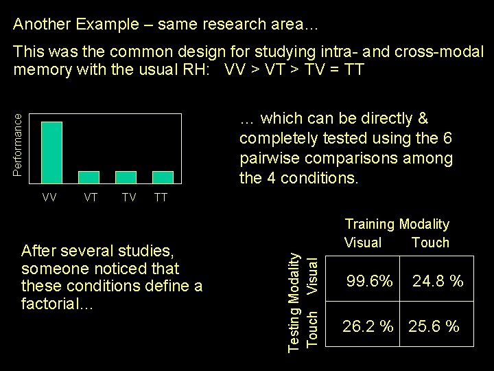
Another Example – same research area… This was the common design for studying intra- and cross-modal memory with the usual RH: VV > VT > TV = TT Performance … which can be directly & completely tested using the 6 pairwise comparisons among the 4 conditions. VT TV TT After several studies, someone noticed that these conditions define a factorial… Training Modality Visual Touch Testing Modality Touch Visual VV 99. 6% 24. 8 % 26. 2 % 25. 6 %

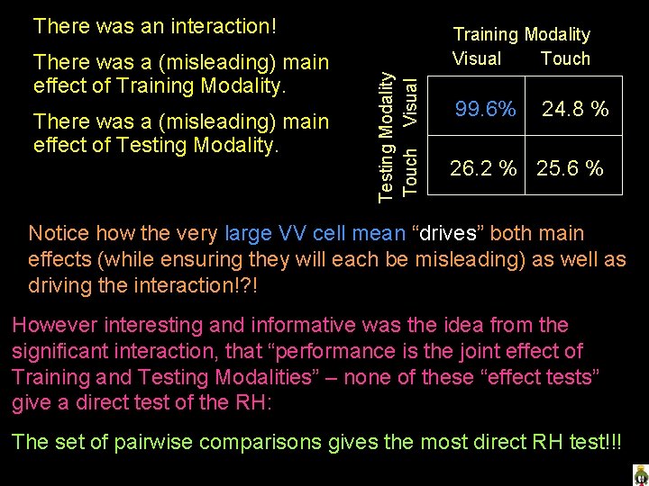
There was an interaction! There was a (misleading) main effect of Testing Modality Touch Visual There was a (misleading) main effect of Training Modality Visual Touch 99. 6% 24. 8 % 26. 2 % 25. 6 % Notice how the very large VV cell mean “drives” both main effects (while ensuring they will each be misleading) as well as driving the interaction!? ! However interesting and informative was the idea from the significant interaction, that “performance is the joint effect of Training and Testing Modalities” – none of these “effect tests” give a direct test of the RH: The set of pairwise comparisons gives the most direct RH test!!!

Here’s yet another way of thinking about interactions… we’ll need an example!! Brownies – great things… worthy of serious theory & research!!! The usual brownie is made with 4 blocks of chocolate and 2 cups of sugar. Replicated research tells us that the average rating of brownies made with this recipe is about 3 on a 10 point scale. My theory? People don’t really like brownies! What they really like is fudge! So, goes my theory, making brownies more “fudge-like” will make them better liked. How to make them more fudge-like, you ask? Add more sugar & more chocolate!!!

So, we made up several batches of brownies and asked people to taste a standardized amount of brownie after rinsing their mouth with water, eating an unsalted saltine cracker and rinsing their mouth a second time. We used the same 10 -point rating scale; 1 = this is the worst plain brownie I’ve ever had, 10=this is the best plain brownie I’ve ever had. Our first study: 2 -cups of sugar 3 So, far so good! 4 -cups of sugar 5

Our second study: What? ? 4 blocks of choc. 3 8 blocks of choc. 2 Oh – yeah! Unsweetened chocolate… Then the argument started. . One side: We have partial support for theory – adding sugar helps, but adding chocolate hurts!!! Other side: We have not tested theory!!! What was our theory? Add more sugar & more chocolate!!! We need a better design!

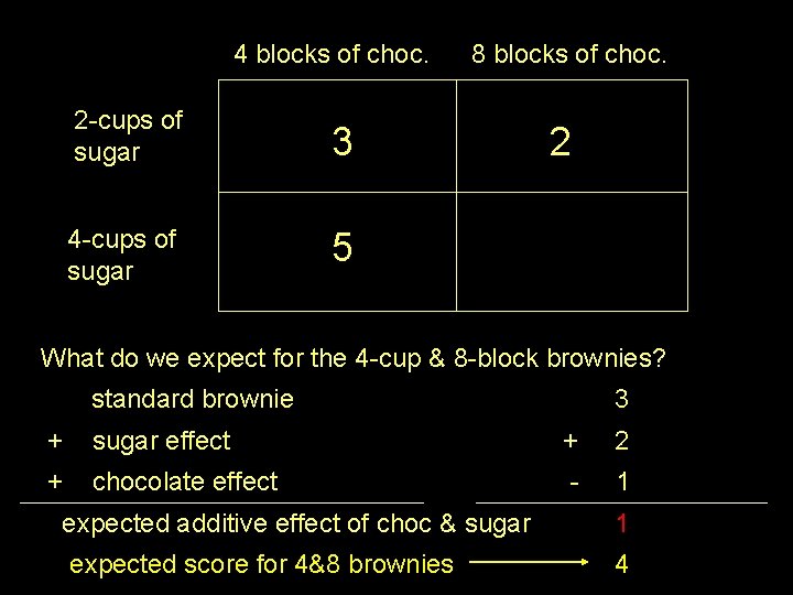
4 blocks of choc. 2 -cups of sugar 3 4 -cups of sugar 5 8 blocks of choc. 2 What do we expect for the 4 -cup & 8 -block brownies? standard brownie 3 + sugar effect + 2 + chocolate effect - 1 expected additive effect of choc & sugar 1 expected score for 4&8 brownies 4

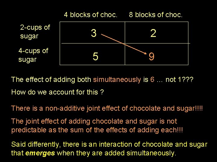
4 blocks of choc. 8 blocks of choc. 2 -cups of sugar 3 2 4 -cups of sugar 5 9 The effect of adding both simultaneously is 6 … not 1? ? ? How do we account for this ? There is a non-additive joint effect of chocolate and sugar!!!! The joint effect of adding chocolate and sugar is not predictable as the sum of the effects of adding each!!! Said differently, there is an interaction of chocolate and sugar that emerges when they are added simultaneously.

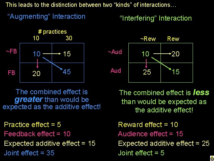
This leads to the distinction between two “kinds” of interactions… “Augmenting” Interaction “Interfering” Interaction # practices 10 30 ~Rew ~FB 10 15 ~Aud 10 20 FB 20 45 Aud 25 15 The combined effect is greater than would be expected as the additive effect! The combined effect is less than would be expected as the additive effect! Practice effect = 5 Feedback effect = 10 Expected additive effect = 15 Joint effect = 35 Reward effect = 10 Audience effect = 15 Expected additive effect = 25 Joint effect = 5

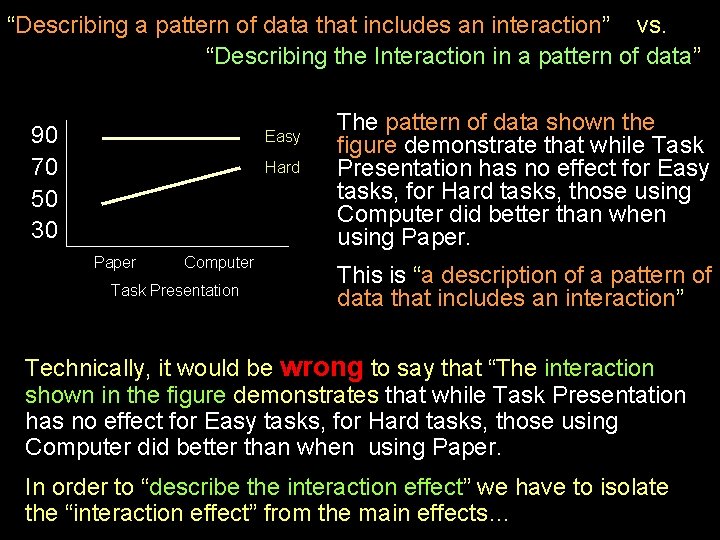
“Describing a pattern of data that includes an interaction” vs. “Describing the Interaction in a pattern of data” 90 70 50 30 Easy Hard Paper Computer Task Presentation The pattern of data shown the figure demonstrate that while Task Presentation has no effect for Easy tasks, for Hard tasks, those using Computer did better than when using Paper. This is “a description of a pattern of data that includes an interaction” Technically, it would be wrong to say that “The interaction shown in the figure demonstrates that while Task Presentation has no effect for Easy tasks, for Hard tasks, those using Computer did better than when using Paper. In order to “describe the interaction effect” we have to isolate the “interaction effect” from the main effects…

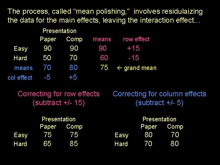
The process, called “mean polishing, ” involves residulaizing the data for the main effects, leaving the interaction effect… Presentation Paper Comp Easy Hard means col effect 90 50 70 -5 90 70 80 +5 means 90 60 75 Correcting for row effects (subtract +/- 15) row effect +15 -15 grand mean Correcting for column effects (subtract +/- 5) Presentation Paper Comp Easy Hard 75 65 75 85 Presentation Paper Comp Easy Hard 80 70 70 80

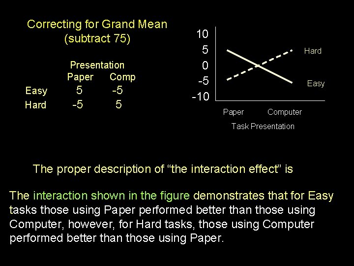
Correcting for Grand Mean (subtract 75) Presentation Paper Comp Easy Hard 5 -5 -5 5 10 5 0 -5 -10 Hard Easy Paper Computer Task Presentation The proper description of “the interaction effect” is The interaction shown in the figure demonstrates that for Easy tasks those using Paper performed better than those using Computer, however, for Hard tasks, those using Computer performed better than those using Paper.

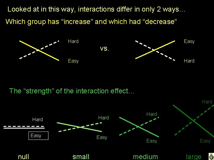
Looked at in this way, interactions differ in only 2 ways… Which group has “increase” and which had “decrease” Hard Easy vs. Easy Hard The “strength” of the interaction effect… Hard Easy null Easy small Hard Easy medium Easy large

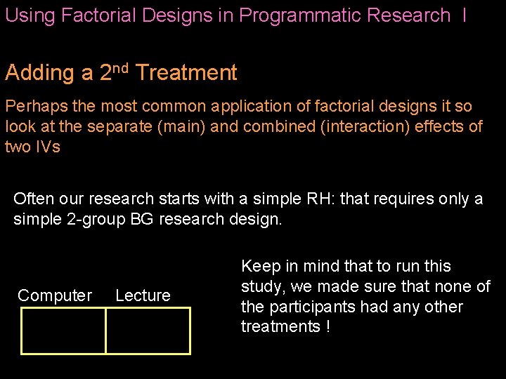
Using Factorial Designs in Programmatic Research I Adding a 2 nd Treatment Perhaps the most common application of factorial designs it so look at the separate (main) and combined (interaction) effects of two IVs Often our research starts with a simple RH: that requires only a simple 2 -group BG research design. Computer Lecture Keep in mind that to run this study, we made sure that none of the participants had any other treatments !

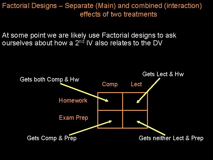
Factorial Designs – Separate (Main) and combined (interaction) effects of two treatments At some point we are likely use Factorial designs to ask ourselves about how a 2 nd IV also relates to the DV Gets both Comp & Hw Gets Lect & Hw Comp Lect Homework Exam Prep Gets Comp & Prep Gets neither Lect & Prep

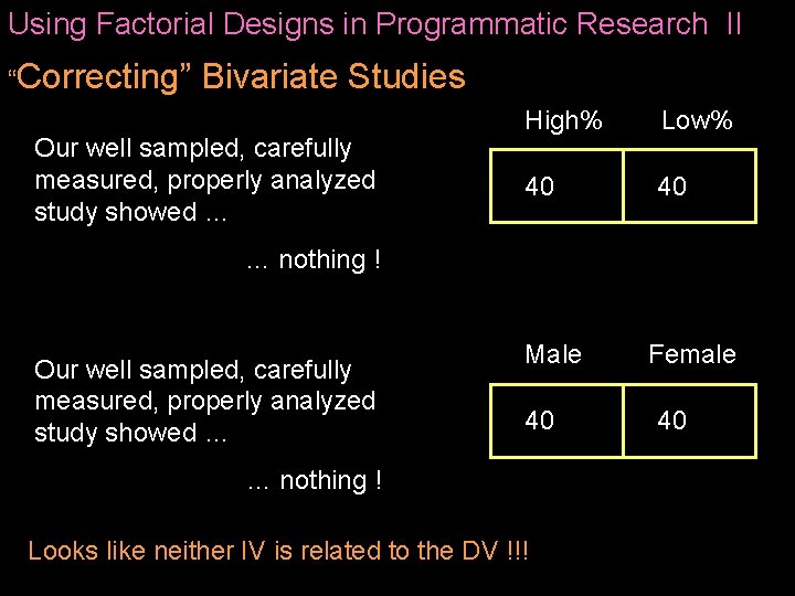
Using Factorial Designs in Programmatic Research II “Correcting” Bivariate Studies Our well sampled, carefully measured, properly analyzed study showed … High% Low% 40 40 … nothing ! Our well sampled, carefully measured, properly analyzed study showed … Male 40 … nothing ! Looks like neither IV is related to the DV !!! Female 40

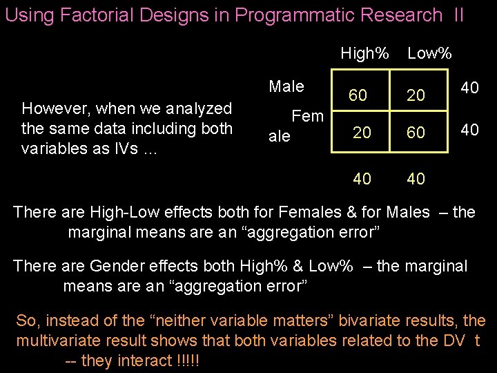
Using Factorial Designs in Programmatic Research II High% Male However, when we analyzed the same data including both variables as IVs … Fem ale Low% 60 20 40 20 60 40 40 40 There are High-Low effects both for Females & for Males – the marginal means are an “aggregation error” There are Gender effects both High% & Low% – the marginal means are an “aggregation error” So, instead of the “neither variable matters” bivariate results, the multivariate result shows that both variables related to the DV t -- they interact !!!!!

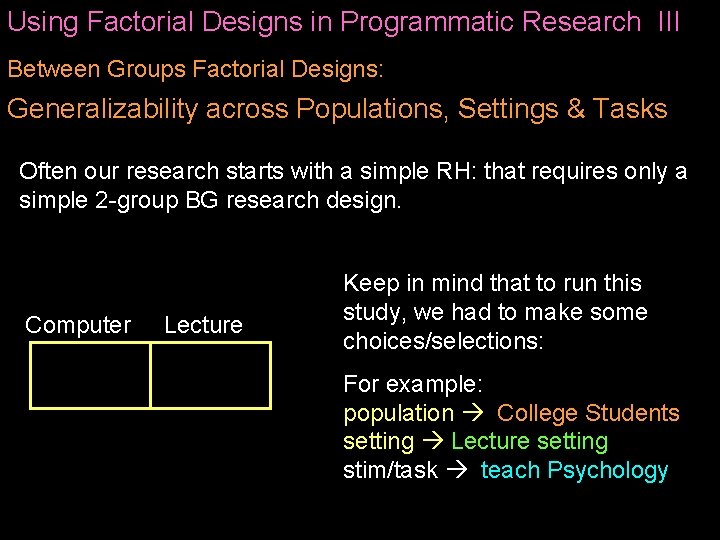
Using Factorial Designs in Programmatic Research III Between Groups Factorial Designs: Generalizability across Populations, Settings & Tasks Often our research starts with a simple RH: that requires only a simple 2 -group BG research design. Computer Lecture Keep in mind that to run this study, we had to make some choices/selections: For example: population College Students setting Lecture setting stim/task teach Psychology

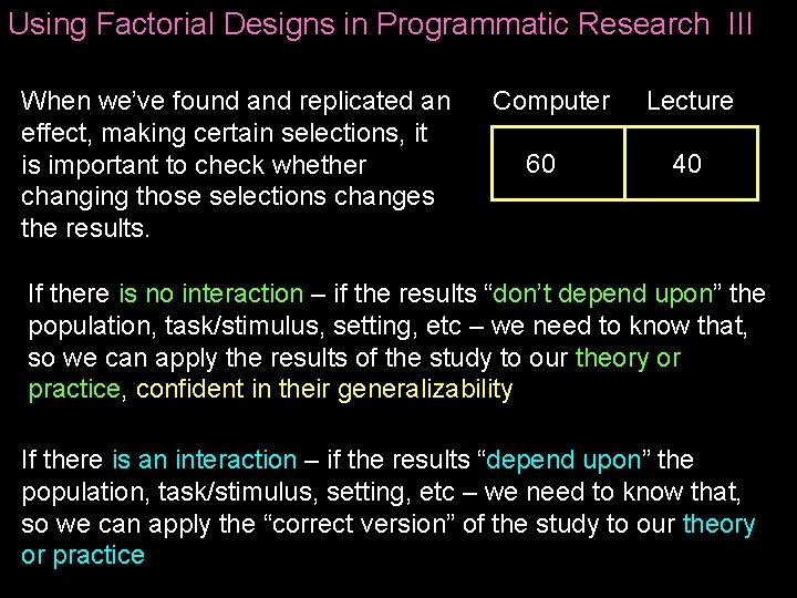
Using Factorial Designs in Programmatic Research III When we’ve found and replicated an effect, making certain selections, it is important to check whether changing those selections changes the results. Computer 60 Lecture 40 If there is no interaction – if the results “don’t depend upon” the population, task/stimulus, setting, etc – we need to know that, so we can apply the results of the study to our theory or practice, confident in their generalizability If there is an interaction – if the results “depend upon” the population, task/stimulus, setting, etc – we need to know that, so we can apply the “correct version” of the study to our theory or practice

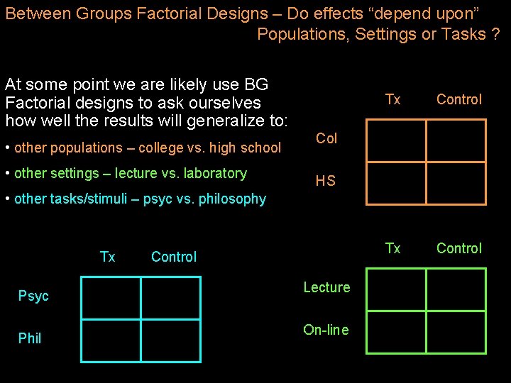
Between Groups Factorial Designs – Do effects “depend upon” Populations, Settings or Tasks ? At some point we are likely use BG Factorial designs to ask ourselves how well the results will generalize to: • other populations – college vs. high school • other settings – lecture vs. laboratory Tx Control Col HS • other tasks/stimuli – psyc vs. philosophy Tx Psyc Phil Control Lecture On-line

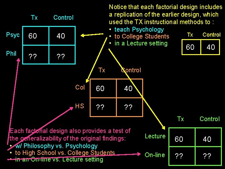
Tx Psyc Phil 60 Notice that each factorial design includes a replication of the earlier design, which used the TX instructional methods to : • teach Psychology Tx Control • to College Students • in a Lecture setting Control 40 60 ? ? 40 ? ? Tx Control Col 60 40 HS ? ? Tx Each factorial design also provides a test of the generalizability of the original findings: • w/ Philosophy vs. Psychology • to High School vs. College Students • in an On-line vs. Lecture setting Control Lecture 60 40 On-line ? ?

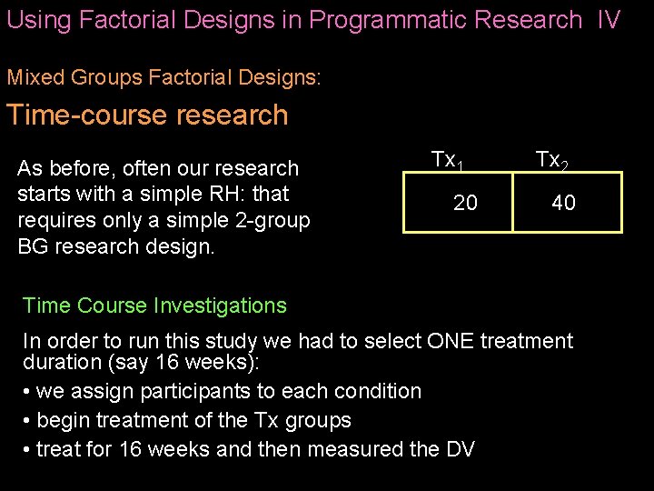
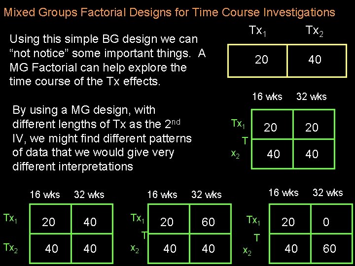
Using Factorial Designs in Programmatic Research IV Mixed Groups Factorial Designs: Time-course research As before, often our research starts with a simple RH: that requires only a simple 2 -group BG research design. Tx 1 20 Tx 2 40 Time Course Investigations In order to run this study we had to select ONE treatment duration (say 16 weeks): • we assign participants to each condition • begin treatment of the Tx groups • treat for 16 weeks and then measured the DV

Mixed Groups Factorial Designs for Time Course Investigations Tx 1 Tx 2 Using this simple BG design we can “not notice” some important things. A 20 40 MG Factorial can help explore the time course of the Tx effects. 16 wks By using a MG design, with different lengths of Tx as the 2 nd IV, we might find different patterns of data that we would give very different interpretations 16 wks Tx 1 20 32 wks 40 16 wks Tx 1 20 Tx 1 40 40 x 2 40 20 20 40 40 T x 2 16 wks 32 wks 60 Tx 1 T Tx 2 32 wks 40 T x 2 32 wks 20 0 40 60

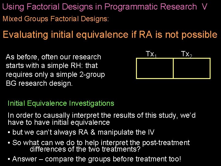
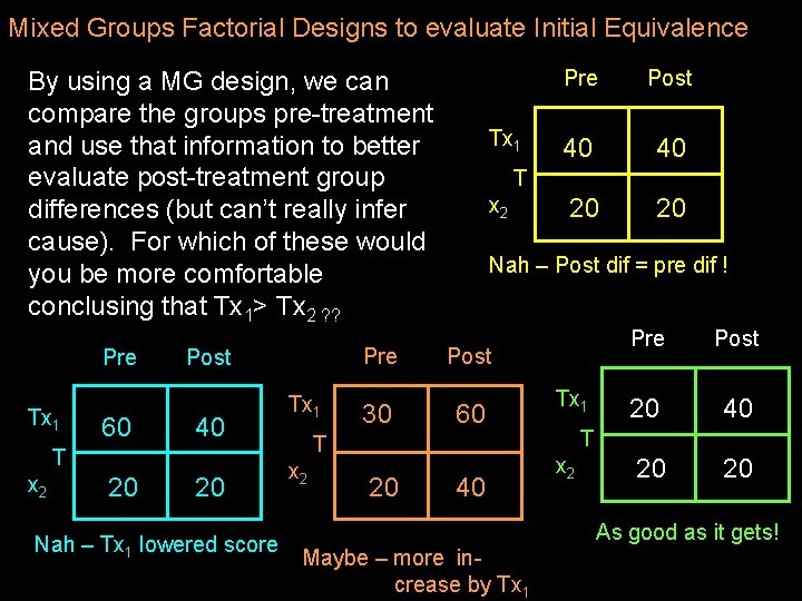
Using Factorial Designs in Programmatic Research V Mixed Groups Factorial Designs: Evaluating initial equivalence if RA is not possible As before, often our research starts with a simple RH: that requires only a simple 2 -group BG research design. Tx 1 Tx 2 Initial Equivalence Investigations In order to causally interpret the results of this study, we’d have to have initial equivalence • but we can’t always RA & manipulate the IV • So what can we do to help interpret the post-treatment differences of the two treatments? • Answer – compare the groups before treatment too!

Mixed Groups Factorial Designs to evaluate Initial Equivalence By using a MG design, we can compare the groups pre-treatment and use that information to better evaluate post-treatment group differences (but can’t really infer cause). For which of these would you be more comfortable conclusing that Tx 1> Tx 2 ? ? Pre Tx 1 60 Post 40 T x 2 20 20 Nah – Tx 1 lowered score Tx 1 x 2 40 40 20 20 Nah – Post dif = pre dif ! Pre Post 30 60 20 Post T T x 2 Pre 40 Tx 1 Pre Post 20 40 20 20 T x 2 As good as it gets! Maybe – more increase by Tx 1