Principle Component Analysis PCA A mechanism used to

Principle Component Analysis (PCA) A mechanism used to make the analysis of remote sensing data simpler….

PCA n n reduces the dimensionality of the data keeping the (what we hope) is the most significant parts of the data simultaneously filters out ‘noise’ It is a way of identifying patterns in data, and expressing the data in such a way as to highlight their similarities and differences

PCA contd. n n n “hyperspace graphing” is not available to visualize data the 3 first principle components make a powerful tool for identifying patterns in the data This is can be seen as a tool for image compression with no loss of information

History… n n n Early image processing systems were limited in their processing capacity… it was important to reduce the number of calculations required to process an image. Currently, useful as tool to explore the variability of an image Also used in facial recognition software

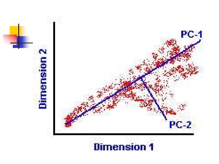
How it works The data, though clumped around several central points in that hyperspace, will generally tend towards one direction. If one were to draw a solid line that best describes that direction, then that line is the first principle component (PC).

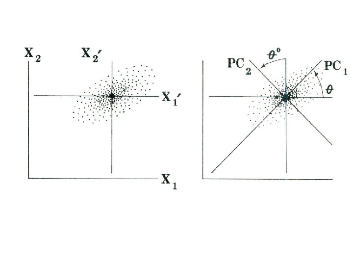
Eigenvectors and Eigenvalues n n n Each eigenvector represents a principle component. The first Principle Component is defined as the eigenvector with the highest corresponding eigenvalue. The individual eigenvalues indicate the variance they capture - the higher the value, the more variance they have captured.

n n Any variation that is not captured by that first PC is captured by subsequent orthogonal eigenvectors. When the data is plotted in this manner they are said to be plotted in Principle Component-space (PC-space)

Data means WHAT? n n n The first PC represents the greatest variability in the data … so? How does the interpreter convert ‘variability’ into information?

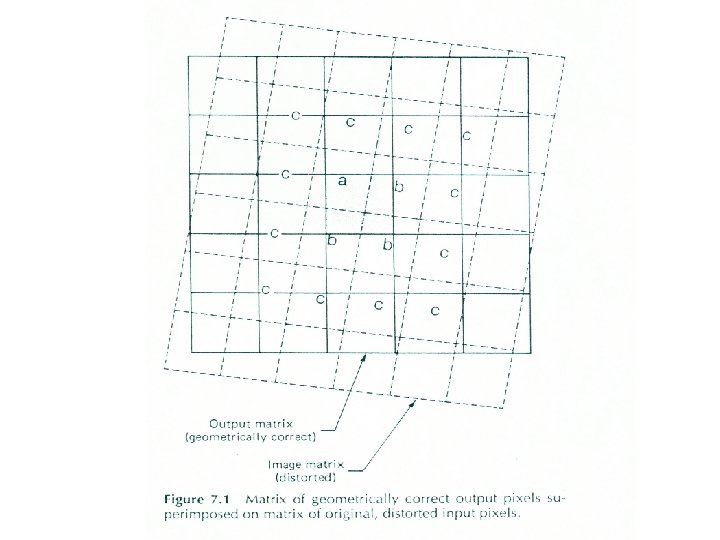
Image Registration and Rectification n n Removing spatial errors in an image Systematic errors n n n (skew) Curvature of the earth General instrument correction e. g. scan line overlap

Projection and Random errors n n In order to get RS data into a format compatible with the GIS, a projection needs to be specified (the alternative is to do an ‘image based’ GIS that ignores real world coordinates)

Ground Control Points (GCPs) n n Use GCPs that are well distributed across the image Features visible on the image that correspond to known locations on the ground (or on a map) GCP 1 - XY (UTM? ) GCP 1 -row/column

Affine Coordinate Transformation n n X =a 0+a 1 X+a 2 Y Y = b 0+b 1 X+b 2 Y Where x and y are the row/ column locations And X, Y are the ground coordinates an and bn are transformation parameters

Page 2 (of 3) of the affine coordinate transformation example in Jensen 1986

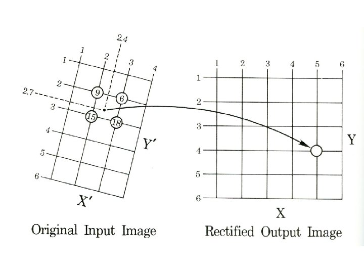
So how do we get new values into the projected cells? n Nearest neighbor n n n The cell value from the original image closest to the center of the new (rectified or projected) cell is assigned to the new cell. Simplest method Only rational method for classified images or other grid data with interval data

Bilinear Interpolation n n Weighted average of the four nearest pixels (2 left-right and 2 up-down) weighted average of a 2 X 2 kernel

Cubic Convolution or Cubic spline n n Cubic spline of 16 closest neighbors a weighted average of from a 4 X 4 kernel

How well do they work? n n n Every manipulation of a grid changes the data in every grid cell The accuracy of the original data ? The accuracy of the ‘new’ cells ? Loss of information ? The only real test of accuracy is how accurately INFORMATION is supplied by the image….

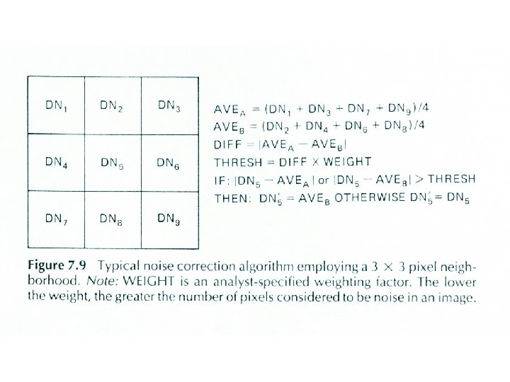
Image Filtering n n n Noise removal Smoothing Edge enhancement Most image enhancement operations work the same way A moving window

The kernel or window n n The factors in the moving window are specified based on the desired result The 3 X 3 array moves across the image and converts the value of the center pixel based on the operations specified by the surrounding pixels

A ‘high pass’ filter or kernel

Directional Edge Enhancement… examples