Pairings on ECC Debdeep Mukhopadhyay Associate Professor Dept

Pairings on ECC Debdeep Mukhopadhyay Associate Professor Dept of Computer Sc and Engg, IIT Kharagpur

Global Definitions • For a field K, nϵN, kϵK, we define: n. k=k+k+…+k (n times) • The characteristic of a field K is defined as: • char(K)= 0 for CK=Φ min(CK) else with CK={pϵN>0|p. 1=0, 1 ϵ K additive neutral} • Proposition 1. 1 char(K) is either 0 or prime.
≠ 2 or")
Algebraically Closed Fields • K is an algebraically closed field with char(K)≠ 2 or 3. • The letters X and Y are variables. • K[X] and K[X, Y] are polynomial rings in one respective two variables. • K(X) and K(X, Y) are the field of rational functions in one respective two variables.
![Elliptic Curves • Vanishing Set: For fϵK[X, Y] we define V(f)={(a, b) ϵ K](http://slidetodoc.com/presentation_image_h2/75765c54f16657217f26b0b81da30bc5/image-4.jpg "Elliptic Curves • Vanishing Set: For fϵK[X, Y] we define V(f)={(a, b) ϵ K")
Elliptic Curves • Vanishing Set: For fϵK[X, Y] we define V(f)={(a, b) ϵ K 2|f(a, b)=0} • Elliptic Curves: E=EA, B=V(Y 2 -X 3 -AX-B)U{O} Is called an elliptic curve over K ifs(x)=s. A, B(x)=x 3+Ax+B has three distinct roots. The elements OϵE is called identity or point at infinity and elements of E{O} finite. • Negative of a point P: (a, -b) also called –P • Discriminant: ∆(EA, B)=-4 A 3 -27 B 2

Non-singular Elliptic Curves • The set EA, B is called an elliptic curve. • The elliptic curve is non-singular iff s. A, B has 3 distinct roots. • Otherwise it is called singular. • We will deal with only non-singular curves. • They are also called smooth curves.
: Singular Cubic Curves Examples of Elliptic")
Singular and non-singular curves y 2=x 3 (Cusp): Singular Cubic Curves Examples of Elliptic Curves: Non-singular Note: The curves are not over finite fields. They are over R, which is not algebraically closed.

Points of Order 2 • Let EA, B be an Elliptic Curve and w 1, w 2, w 3 the three distinct roots of s. A, B(x). • The three points Ωi=(wi, 0) ϵ EA, B are called points of order two. • Since K is algebraically closed f(x)=(x-w 1)(x-w 2)(x-w 3)=x 3+Ax+B • The set EA, B is an elliptic curve iff ∆(EA, B)≠ 0.
={(a, b)ϵEA, B|a, bϵk}∪{O}")
k-rational points • For a subfield k⊆K and A, Bϵk E(k)={(a, b)ϵEA, B|a, bϵk}∪{O} are called k-rational points. • More generic definition: • A plane affine curve C over K is defined by a non-zero polynomial as C: f(X, Y)=0 • A K-rational point on a curve C : f(X, Y)=0 is a point P=(h, k)ϵK 2 such that f(P)=f(h, k)=0.
![Polynomials on Elliptic Curves • For two polynomials G(X, Y) and H(X, Y)ϵK[X, Y]](http://slidetodoc.com/presentation_image_h2/75765c54f16657217f26b0b81da30bc5/image-9.jpg "Polynomials on Elliptic Curves • For two polynomials G(X, Y) and H(X, Y)ϵK[X, Y]")
Polynomials on Elliptic Curves • For two polynomials G(X, Y) and H(X, Y)ϵK[X, Y] with f|(G-H) we have G(P)=H(P) for every rational point P on the curve C. • Thus G and H represent the same K-valued function on C. • Thus we can define a congruence: • G(X, Y)≡H(X, Y) (mod f(X, Y)) iff f|(G-H) • We define the co-ordinate ring of C: • K[C]=K[X, Y]/<f(X, Y)> • We define G(x, y) as the equivalence class of a polynomial G(X, Y)ϵK[X, Y]. • The set of fractions of elements of K[C] with non-zero denominators is a field denoted as: • K(C)={G(x, y)/H(x, y)|H(x, y)≠ 0} • K(C) is called the function field of C.

Application to an EC • Consider an elliptic curve EA, B : Y 2=X 3+AX+B=s(X). • Let the small letters x and y be the co-ordinate functions, x(a, b)=a and y(a, b)=b on E. • Thus E satisfied y 2=s(x). • With this notation we can say K[E]=K[x, y]. • How can we thus obtain the congruences? • Replace every Y 2 in a polynomial f ϵK[X, Y] by the term X 3+AX+B • This does not change the equivalence class of f. • So any f can be written as f(x, y)=v(x)+yw(x) with v, wϵK[X, Y • We denote the set of polynomials on E by: K[E]=K[X, Y]/(Y 2 -X 3 -AX-B)
=y 4+x 2 y+x+1 =(y 2)2+x 2 y+x+1 =(x 3+Ax+B)2+x 2")
Example • F(x, y)=y 4+x 2 y+x+1 =(y 2)2+x 2 y+x+1 =(x 3+Ax+B)2+x 2 y+x+1 =[(x 3+Ax+B)2+x+1]+y[x 2] V(x) w(x)
![Canonical Forms • A polynomial f ϵK[X, Y] is said to be written in](http://slidetodoc.com/presentation_image_h2/75765c54f16657217f26b0b81da30bc5/image-12.jpg "Canonical Forms • A polynomial f ϵK[X, Y] is said to be written in")
Canonical Forms • A polynomial f ϵK[X, Y] is said to be written in canonical forms when we write f(x, y)=v(x)+yw(x). • The canonical form is unique! • Let f(x, y)=v 1(x)+yw 1(x)=v 2(x)+yw 2(x) be two canonical forms. • Thus, (v 1(x)-v 2(x))+y(w 1(x)- w 2(x))=0. • Setting, v(x)= v 1(x)-v 2(x), w(x)= w 1(x)- w 2(x), we have v(x)+yw(x)=0. • Thus, 0=(v(x)+yw(x))(v(x)-yw(x))=v 2(x)-y 2 w 2(x) = v 2(x)-(s(x))w 2(x). • Note, degx(v 2(x)) and degx(w 2(x)) is even. But degx(s(x)) is odd. Thus, the polynomial w(x) is 0, hence v(x) is also 0.

Conjugate and Norm •

Rational Functions on EC •

Canonical form for Rational Functions •

Rational Functions at O •
![Connection of degree to Classical degree • For fϵK[E], deg(f)=degx(Nf) • Write f in](http://slidetodoc.com/presentation_image_h2/75765c54f16657217f26b0b81da30bc5/image-17.jpg "Connection of degree to Classical degree • For fϵK[E], deg(f)=degx(Nf) • Write f in")
Connection of degree to Classical degree • For fϵK[E], deg(f)=degx(Nf) • Write f in canonical form: f(x, y)=v(x)+yw(x). • Then Nf=v 2(x)-s(x)w 2(x). • Thus, degx(Nf)=degx(v 2(x)-s(x)w 2(x)) =max{degx(v 2), degx(s)+degx(w 2)) =max{2. degx(v), 3+2. degx(w)} =deg(f)
![Property of Degree of Polynomials • For f, gϵK[E], deg(f. g)=deg(f)+deg(g) • From the](http://slidetodoc.com/presentation_image_h2/75765c54f16657217f26b0b81da30bc5/image-18.jpg "Property of Degree of Polynomials • For f, gϵK[E], deg(f. g)=deg(f)+deg(g) • From the")
Property of Degree of Polynomials • For f, gϵK[E], deg(f. g)=deg(f)+deg(g) • From the previous result, deg(f. g)=degx(Nfg) =degx(Nf. Ng) =degx(Nf)+degx(Ng) =deg(f)+deg(g)

Evaluating a rational function at O •

An Example •

An Example •
 st. r(O) and s(O) are finite then")
Some more propositions • For r, sϵK(E) st. r(O) and s(O) are finite then it holds that: (r. s)(O)=r(O)s(O) (r+s)(O)=r(O)+s(O)
. • Zero: We say that r has")
Zeros, Poles, and Uniformizers • Let rϵK(E). • Zero: We say that r has a zero at PϵE if r(P)=0 • Pole: We say that r has a pole at P if r(P) is not finite. • Determining poles and zeros can be tricky. Consider the unit circle C: X 2+Y 2 -1=0. Consider R(x, y)=(1 -x)/y ϵK(C). Take P=(1, 0). Plugging, R(x, y) gives the form 0/0 and it appears R is not defined at P. • But take a second look! • •

Zeros, Poles, and Uniformizers •

Uniformizers •

Uniformizer in general case •

Decomposing f=uds •

Decomposing f=uds •

Termination Proof •

Uniformizer at points with order two. •

Uniformizer at O •

Uniformizer Theorem • Every point on an EC has a uniformizer and the number d does not depend on its choice. • The existence is already shown. • We are to show that d does not depend on its choice. • Let u and u’ be uniformizers at P • Thus, u=u’aq, and u’=ubp, for a, bϵZ, q, pϵK(E) are both finite and non-zero at P. • Thus, u=u’aq=(ubp)aq=uab(paq). • Assume, ab≠ 1, thus 1=uab-1(paq). Thus evaluated at P, we have 1=0. • Hence, a=b=± 1. • If a=b=-1, u=u’-1 q=>uu’=q. Evaluated at P this leads to a contradiction, since 0=u(P)u’(P)=q(P) ≠ 0. • Thus a=b=1.
{0} be arbitrary. Since, u and u’ are uniformizers, Эd,")
Proof Contd. • Let rϵK(E){0} be arbitrary. Since, u and u’ are uniformizers, Эd, d’ and s, t ϵK(E){0} finite and nonzero at P st. r=uds, and r=u’d’t. • uds=u’d’t=(up)d’t=ud’(pd’t)=>ud-d’=pd’t/s • On the right hand side, we have rational functions which are non-zero at P. • But on the left hand side, we have zero if d-d’≠ 0. • Thus, d=d’ • Because, of the independence of d from u we can define the order of a rational function.

Order of a Rational Function • For an elliptic E let PϵE be a point and u an uniformizer at P. For rϵK(E){0} with r=uds, we call d the order of r at P, and write ord. P(r)=d. • The multiplicity of a zero is the order of r at that zero point. • The multiplicity of a pole is the negative of the order of r at that point.

Order of a Zero • If the zero does not correspond to a point of order two: • Let f be a function fϵK[X] with f(x)=g(x)(x-a)k for gϵK[X] with g(a)≠ 0, kϵN>0 and aϵK. • Now see f as a polynomial fϵK[E] and pick a uniformizer at P=(a, ±s(a)1/2) (zero of f) • u=(x-a) • S(x, y)=g(x) • Then d=k=ordf(P)
, P=(a, 0)")
Zero is a point of order two • When a=wi (wlog i=1), P=(a, 0) is a zero. • Uniformizer: u(x, y)=y at P. Note u(P)=0. • s(x, y)=g(x)/(x-w 2)k(x-w 3)k • We write f(x, y)=uds(x, y)=ydg(x)/(x-w 2)k(x-w 3)k = yd [(x-a)kg(x)/(x-w 1)k(x-w 2)k(x-w 3)k] =yd [(x-a)kg(x)/y 2 k]=>d=2 k
 and PϵE, st. r(P)≠ 0 and")
Order of a finite non-root • Let rϵK(E) and PϵE, st. r(P)≠ 0 and r is finite at P then ord. P(r)=0 • Set, d=0 and s=r
![Order of Polynomials at O • For fϵK[E]{0} and ord. O(f)=-deg(f) • • Let](http://slidetodoc.com/presentation_image_h2/75765c54f16657217f26b0b81da30bc5/image-38.jpg "Order of Polynomials at O • For fϵK[E]{0} and ord. O(f)=-deg(f) • • Let")
Order of Polynomials at O • For fϵK[E]{0} and ord. O(f)=-deg(f) • • Let u=x/y be a uniformizer at O. Let k=deg(f), we take s(x, y)=(xk/yk)f(x, y). deg(xkf(x, y))=2 k+deg(f)=3 k deg(yk)=3 k • Thus s is finite and non-zero • Thus from f(x, y)=(x/y)d(xk/yk)f(x, y)=>d=-k
, and PϵE,")
Property of Order of Rational Functions • For r 1, r 2ϵK(E), and PϵE, ord. P(r 1. r 2)=ord. P(r 1)+ord. P(r 2) • Let PϵE and pick a uniformizer u at P. • Thus we have: r 1. r 2=uds, r 1=ud 1 s 1, r 2=ud 2 s 2. • Thus, ud. s=r 1 r 2=(ud 1 s 1)(ud 2 s 2). • Since, s, s 1, s 2 are non-zero rational functions we have d=d 1+d 2. • This proves the result.
=x-a, where s(a)")
Examples • We now want to calculate the orders of r(x, y)=x-a, where s(a) ≠ 0 for all points QϵE where r(Q) is not finite or zero • ie. at all other points ord. Q(r)=0 • Zeros: Clearly, when x=a, r(Q=P)=0. Thus the zero is at (a, b) where b ≠ 0 (since s(a)≠ 0). • Assume Q=P or Q=P’=(a, -b)≠ 0. Take r itself as the uniformizer, ie. r=r 1. 1, and ord. Q(r)=d=1. • Poles: Take u=x/y as the uniformizer. r=(x-a), deg(r)=2. Thus (x-a)=(x/y)-2[(x/y)2(x-a)]. Thus, ord. Q(r)=-2. • Summing up, two zeros of order 1, and one pole of order -2.
=0, there is only one zero, viz, say (w 1,")
Example • Note when s(a)=0, there is only one zero, viz, say (w 1, 0). • What is the order of zero?
=0, there is only one zero, viz, say (w 1,")
Example • Note when s(a)=0, there is only one zero, viz, say (w 1, 0), where a=w 1. • What is the order of zero? • (x-a)=yd (1/(x-w 2)(x-w 3))=yd [(x-a)/(x-w 1)(x-w 2)(x-w 3)] =yd-2(x-a) • Hence, d=2. • Thus, we have a zero with order 2 and a pole with order -2.
=y • Zeros: The zeros are at y=0, which are")
Examples • Let r(x, y)=y • Zeros: The zeros are at y=0, which are points of order two. • Thus, u(x, y)=y is the unformizer at the three zeros Qi=(wi, 0), i=1, 2, 3. We have ord. Q(r)=1. • At every other finite point order is 0. • Pole: Now consider the pole at point O. Note deg(r)=3. Hence, d=-3, u(x, y)=x/y, and s(x, y)=(x/y)3 y=x 3 y/y 3. • Note deg(s)=2. 3+3 -3. 3=0, hence s is finite at O. • Thus we have 3 zeros with order 1, and one pole with order -3.
-deg(y)=2 -3=-1<0, ie.")
Example • Consider r=x/y. • Zeros: • Point at O: • deg(x)-deg(y)=2 -3=-1<0, ie. r(O)=0. • u(x, y)=x/y • (x/y)=(x/y)1. 1=> ord. O(r)=1. • x=0, P±=(0, ±B 1/2) are zeros of r, where B≠ 0. • u(x, y)=x • (x/y)=xd(1/y), note s(x, y)=1/y is finite and non-zero at P±. • Thus, ord. P±(r)=1. • Poles: r is not finite when y=0. • Points of order two, Qi=(wi, 0) • u(x, y)=y • (x/y)=y-1(x), note s(x, y)=x is finite and non-zero at Qi, as B≠ 0, and w 1 w 2 w 3=-B, hence wi’s≠ 0. • Thus, we have three zeros with order 1 and three pole with order -1.
 • Note the simple zero at O remains. • For the")
Example (Case B=0) • Note the simple zero at O remains. • For the others we recalculate: • y 2=x 3+Ax=x(x-(-A)1/2)(x+(-A)1/2) • Thus w 1=0, w 2=(-A)1/2, w 3=-(-A)1/2 are three points of order two. • Note w 2 and w 3 are poles as before, but not w 1. • At w 2 and w 3, we have (x/y)=ydx, again d=-1. • At w 1=0. , ie, (0, 0) we observe • (x/y)=xy/y 2=xy/(x(x-(-A)1/2)(x+(-A)1/2))=y/(x-(-A)1/2)(x+(-A)1/2)=0 • Thus we have a zero at w 1. • Order? • Take u=y, s=1/(x-(-A)1/2)(x+(-A)1/2), note s is finite and non-zero at w 1=0. • Thus, y/(x-(-A)1/2)(x+(-A)1/2)=yd(1/(x-(-A)1/2)(x+(-A)1/2), and hence d=1 • We have two zeros with order one and two poles with order -1.

Baby Riemann Roch Theorem •

Sum of Order is Zero •

Rational Maps and Endomorphisms •

Rational Map •

Examples of Maps •

Isomorphisms • A rational map α: E->E is called an endomorphism or isogeny of E if α is a group homomorphism, ie. α(P+Q)= α(P)+ α(Q), for all P, QϵE. • A bijective isogeny is called isomorphism.

Torsion Points •

Formal Sum •

Divisor •

Divisors of a Rational Function •

Picard Group •
![Example: Zeros and Poles of Straight Lines • Div(L)=[P]+[Q]+[R]-3[O] • Div(T)=2[P]+[Q]-3[O] • Div(V)=[P]+[Q]-2[O]](http://slidetodoc.com/presentation_image_h2/75765c54f16657217f26b0b81da30bc5/image-57.jpg "Example: Zeros and Poles of Straight Lines • Div(L)=[P]+[Q]+[R]-3[O] • Div(T)=2[P]+[Q]-3[O] • Div(V)=[P]+[Q]-2[O]")
Example: Zeros and Poles of Straight Lines • Div(L)=[P]+[Q]+[R]-3[O] • Div(T)=2[P]+[Q]-3[O] • Div(V)=[P]+[Q]-2[O]

Principal Divisor •

Divisors of a line and vertical line •
,")
Example • E: Y 2=X 3+X+5 defined over F 37. • Take P=(1, 9), Q=(10, 4). • Equation of LP, Q: y=((4 -9)/(10 -1))x+c=20 x+c, where c=26=> LP, Q: y+17 x+11=0 • The line meets the curve at R=(19, 36), -R=(19, 36)=(19, 1). • Vertical line: LR, -R: x-19=0, ie. x+18=0 • Div(y+17 x+11/x+18)=([P]-[O])-([P+Q]-[Q])

Evaluate a rational function at a Divisor •
 is invariant upto multiplications by constants •")
f(D) is invariant upto multiplications by constants •

Weil’s Reciprocity Theorem • If f and g are two non-zero rational functions on E and Div(f) and Div(g) have disjoint supports, f(Div(g))=g(Div(f)). • I will not prove this result but shall give an example.
=y+17 x+11")
Example • E: Y 2=X 3+X+5 defined over F 37 • f(x, y)=y+17 x+11 • Div(f)=[P 1]+[P 2]+[P 3]-3[O], where P 1=(1, 9), P 2=(10, 4), P 3=(19, 36) • g(x, y)=(x+16)/(x+4): • Zero: P 4=(-16, 0)=(21, 0), order is 2. • Pole: P 5=(-4, 14)=(33, 14), P 6=(-4, -14)=(33, 23), order is 1. • Div(g)=2[P 4]-[P 5]-[P 6] (Note at O the function is 1, so it is not in the support of g) • Div(f) and Div(g) are thus disjoint. • f(Div(g))=f(P 4)2 f(P 5)-1 f(P 6)-1=35231 -13 -1=8 (mod 37) • g(Div(f))=g(P 1)g(P 2)g(P 3)g(O)-3=33. 23. 16. 1 -3=8 (mod 37)

Pairings on EC •

Weil Pairing •

Weil Pairing is independent of D 1 and D 2 •

An Alternative Form •

Weil Pairing •
 is independent of the choice of the")
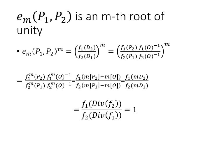
Properties of Weil Pairing • em(P, Q) is independent of the choice of the functions and the point S. • The value of em(P, Q) is an mth root of unity. • The Weil Pairing is bilinear in a multiplicative manner: • em(P 1+P 2, Q)=em(P 1, Q)em(P 2, Q) • em(Q, P 1+P 2)=em(Q, P 1)em(Q, P 2) • Alternating: em(P, P)=1 • Skew-symmetric: em(P, Q)=em(Q, P)-1 • Non-degenerate: If em(P, Q)=1 for all QϵE[m], then P=O.

Proof of Bilinearity •

Proof of Bilinearity •

Proof of Bilinearity •

Miller’s Theorem •

Proof •

Geometry of h. P, Q
 • Let m=m 0+2 m 1+…+2 n")
Miller’s Algorithm • To Compute em(P, Q) • Let m=m 0+2 m 1+…+2 n 1 m n-1 • Following algorithm computes function f. P, st. Div(f. P)=m[P]-[m. P]-(m 1)[O]. • Thus, if PϵE[m], Div(f. P)=m[P]-m[O]
, n=2, ie. n-2=0) • f=f 2 h. P, P=h.")
Proof Idea • Let m=2=(10), n=2, ie. n-2=0) • f=f 2 h. P, P=h. P, P • Note: Div(h. P, P)=2[P]-[2 P]-[O] (which is the desired result).
 • i=0. However step 5 is now executed. •")
Proof Idea • Let m=3=(11) • i=0. However step 5 is now executed. • Thus, f=h. P, Ph 2 P, P • Div(f)=Div(h. P, P)+Div(h 2 P, P) =2[P]-[2 P]-[O]+[2 P]+[P]-[3 P][O]=3[P]-[3 P]-2[O]
 • i=1. Loop executed twice. • Thus, f=(h. P,")
Proof Idea • Let m=4=(100) • i=1. Loop executed twice. • Thus, f=(h. P, P)2 h 2 P, 2 P • Div(f)=2 Div(h. P, P)+Div(h 2 P, 2 P) =2(2[P]-[2 P]-[O])+([2 P]+[2 P][4 P]-[O])=4[P]-[4 P]-3[O]

The Final Step! •
- Slides: 82