Overview of machine learning for computer vision T11

Overview of machine learning for computer vision T-11 Computer Vision University of Ioannina Christophoros Nikou Images and slides from: James Hayes, Brown University, Computer Vision course D. Forsyth and J. Ponce. Computer Vision: A Modern Approach, Prentice Hall, 2003.

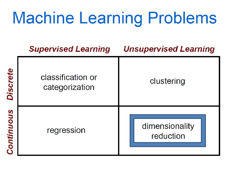
Machine learning: Overview • Core of ML: Making predictions or decisions from Data. • This overview will not go in to depth about the statistical underpinnings of learning methods. • We will explore some algorithms in depth in later classes

Impact of Machine Learning • Machine Learning is arguably the greatest export from computing to other scientific fields.

Machine Learning Applications Slide: Isabelle Guyon

Image Categorization Training Images Image Features Training Labels Classifier Training Classifier parameters

Image Categorization Training Images Image Features Training Labels Classifier Training Classifier parameters Testing Image Features Test Image Trained Classifier Prediction Outdoor

Example: Scene Categorization • Is this a kitchen?

Image features Training Images Image Features Training Labels Classifier Training Trained Classifier

General Principles of Representation • Coverage – Ensure that all relevant info is captured • Concision – Minimize number of features without sacrificing coverage • Directness – Ideal features are independently useful for prediction

Image representations • Templates – Intensity, gradients, etc. • Histograms – Color, texture, SIFT descriptors, etc.

Classifiers Training Images Image Features Training Labels Classifier Training Traine d Classifi er

Learning a classifier Given some set of features with corresponding labels, learn a function to predict the labels from the features x x o x x x o o o x 2 x 1 o x x x

Many classifiers to choose from • • • SVM Neural networks Naïve Bayesian network Logistic regression Randomized Forests Boosted Decision Trees K-nearest neighbor RBMs Etc. Which is the best one?

One way to think about it… • Training labels dictate that two examples are the same or different, in some sense • Features and distance measures define visual similarity • Classifiers try to learn weights or parameters for features and distance measures so that visual similarity predicts label similarity

Claim: The decision to use machine learning is more important than the choice of a particular learning method. If you hear somebody talking of a specific learning mechanism, be wary (e. g. You. Tube comment "Oooh, we could plug this into a Neural network and blah“)

Dimensionality Reduction • PCA, ICA, LLE, Isomap • PCA is the most important technique to know. It takes advantage of correlations in data dimensions to produce the best possible lower dimensional representation, according to reconstruction error. • PCA should be used for dimensionality reduction, not for discovering patterns or making predictions. Don't try to assign semantic meaning to the bases.

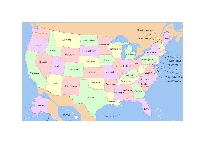
• http: //fakeisthenewreal. org/reform/

• http: //fakeisthenewreal. org/reform/

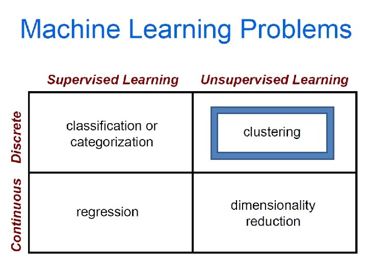
Clustering example: image segmentation Goal: Break up the image into meaningful or perceptually similar regions

Segmentation for feature support 50 x 50 Patch Slide: Derek Hoiem

Segmentation for efficiency [Felzenszwalb and Huttenlocher 2004] [Hoiem et al. 2005, Mori 2005] [Shi and Malik 2001] Slide: Derek Hoiem

Segmentation as a result Rother et al. 2004

Types of segmentations Oversegmentation Undersegmentation Multiple Segmentations

Major processes for segmentation • Bottom-up: group tokens with similar features • Top-down: group tokens that likely belong to the same object [Levin and Weiss 2006]

• Goals Application: Interactive segmentation – User cuts an object to paste into another image – User forms a matte to cope with e. g. hair • weights between 0 and 1 to mix pixels with background • Interactions – mark some foreground, background pixels with strokes – put a box around foreground • Technical problem – allocate pixels to foreground/background class – consistent with interaction information – segments are internally coherent and different from one another

Application: Interactive segmentation

Application: Interactive segmentation

Application: Interactive segmentation

Application: Forming image regions • Pixels are too small and too detailed a representation for – recognition – establishing correspondences in two images – … • Superpixels – Small groups of pixels that are – clumpy, coarse – similar – a reasonable representation of the underlying pixels

Application: Forming image regions

Application: Forming image regions Superpixels

Clustering: group together similar points and represent them with a single token Key Challenges: 1) What makes two points/images/patches similar? 2) How do we compute an overall grouping from pairwise similarities? Slide: Derek Hoiem

Why do we cluster? • Summarizing data – Look at large amounts of data – Patch-based compression or denoising – Represent a large continuous vector with the cluster number • Counting – Histograms of texture, color, SIFT vectors • Segmentation – Separate the image into different regions • Prediction – Images in the same cluster may have the same labels Slide: Derek Hoiem

How do we cluster? • K-means – Iteratively re-assign points to the nearest cluster center • Agglomerative clustering – Start with each point as its own cluster and iteratively merge the closest clusters • Divisive clustering – Start with the whole set of points as one cluster and iteratively generate more clusters • Mean-shift clustering – Estimate modes of pdf • Spectral clustering – Split the nodes in a graph based on assigned links with similarity weights

Clustering for Summarization Goal: cluster to minimize intra-class variance (dispersion) – Preserve information Cluster center Data Whether xj is assigned to ci Slide: Derek Hoiem

K-means algorithm 1. Randomly select K centers 2. Assign each point to nearest center 3. Compute new center (mean) for each cluster Illustration: http: //en. wikipedia. org/wiki/K-means_clustering

K-means algorithm 1. Randomly select K centers 2. Assign each point to nearest center 3. Compute new center (mean) for each cluster Illustration: http: //en. wikipedia. org/wiki/K-means_clustering Back to 2

K-means 0 1. Initialize cluster centers: c ; t=0 2. Assign each point to the closest center 3. Update cluster centers as the mean of the points 4. Repeat 2 -3 until no points are re-assigned (t=t+1) Slide: Derek Hoiem

K-means converges to a local minimum

K-means: design choices • Initialization – Randomly select K points as initial cluster center – Or greedily choose K points to minimize residual • Distance measures – Traditionally Euclidean, could be others • Optimization – Will converge to a local minimum – May want to perform multiple restarts

K-means clustering using intensity or color Image Clusters on intensity Clusters on color

How to choose the number of clusters? • Minimum Description Length (MDL) principal for model comparison • Minimize Schwarz Criterion – also called Bayes Information Criteria (BIC)

How to evaluate clusters? • Generative – How well are points reconstructed from the clusters? • Discriminative – How well do the clusters correspond to labels? • Purity – Note: unsupervised clustering does not aim to be discriminative Slide: Derek Hoiem

How to choose the number of clusters? • Validation set – Try different numbers of clusters and look at performance • When building dictionaries (discussed later), more clusters typically work better Slide: Derek Hoiem

K-means demos • Information and visualization http: //informationandvisualization. de/blog/kmeansand-voronoi-tesselation-built-processing/demo • Alessandro Giusti home – Clustering http: //www. leet. it/home/lale/joomla/component/optio n, com_wrapper/Itemid, 50/ • University of Leicester http: //www. math. le. ac. uk/people/ag 153/homepage/ Kmeans. Kmedoids/Kmeans_Kmedoids. html

K-Means for Segmentation • Pros – Simple and fast method. – Converges to a local minimum. • Cons – Memory-intensive. – Need to pick K. – Sensitive to initialization. – Sensitive to outliers. – Finds “spherical” clusters.

Building Visual Dictionaries 1. Sample patches from a database – E. g. , 128 dimensional SIFT vectors 2. Cluster the patches – Cluster centers are the dictionary 3. Assign a codeword (number) to each new patch, according to the nearest cluster

Examples of learned codewords Most likely codewords for 4 learned “topics” http: //www. robots. ox. ac. uk/~vgg/publications/papers/sivic 05 b. pdf Sivic et al. ICCV 2005