OST Chapter 5 Cellular Manufacturing Group Technology c

OST: Chapter 5 Cellular Manufacturing Group Technology (c) Prof. Richard F. Hartl OST 1

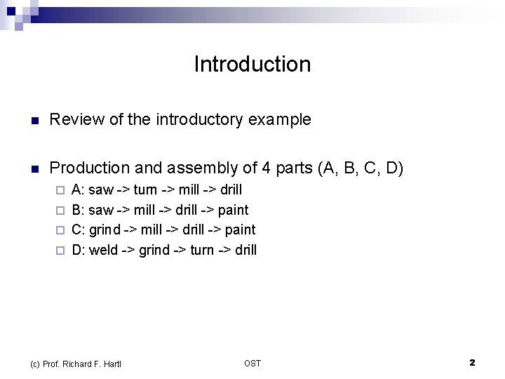
Introduction n Review of the introductory example n Production and assembly of 4 parts (A, B, C, D) A: saw -> turn -> mill -> drill ¨ B: saw -> mill -> drill -> paint ¨ C: grind -> mill -> drill -> paint ¨ D: weld -> grind -> turn -> drill ¨ (c) Prof. Richard F. Hartl OST 2

Group Technology (GT) n n Observation already in 1920 ies: product-oriented departments to manufacture standardized products in machine companies lead to reduced transportation Can be considered the start of Group Technology (GT): Parts with similar features are manufactured together with standardized processes small "focused factories" are created as independent operating units within large facilities. More generally, GT can be considered a “theory of management” based on the principle "similar things should be done similarly“ "things". . product design, process planning, fabrication, assembly, and production control (here); but also other activities, including administrative functions. (c) Prof. Richard F. Hartl OST 3

When to use GT? n n n Pure item flow lines are possible, if volumes are very large. If volumes are very small, and parts are very different, a functional layout (job shop) is usually appropriate In the intermediate case of medium-variety, mediumvolume environments, group configuration is most appropriate (c) Prof. Richard F. Hartl OST 4

Cellular Manufacturing n n Principle of GT: divide the manufacturing facility into small groups or cells of machines cellular manufacturing Each cell is dedicated to a specified family of part types (or few “similar” families). ¨ Preferably, all parts are completed within one cell ¨ n Typically, it consists of ¨ a small group of machines, tools, and handling equipment (c) Prof. Richard F. Hartl OST 5

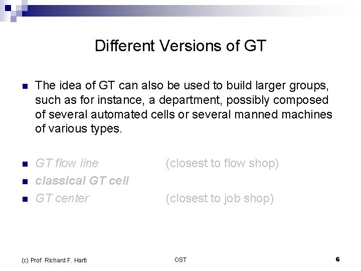
Different Versions of GT n The idea of GT can also be used to build larger groups, such as for instance, a department, possibly composed of several automated cells or several manned machines of various types. n GT flow line classical GT cell GT center n n (c) Prof. Richard F. Hartl (closest to flow shop) (closest to job shop) OST 6

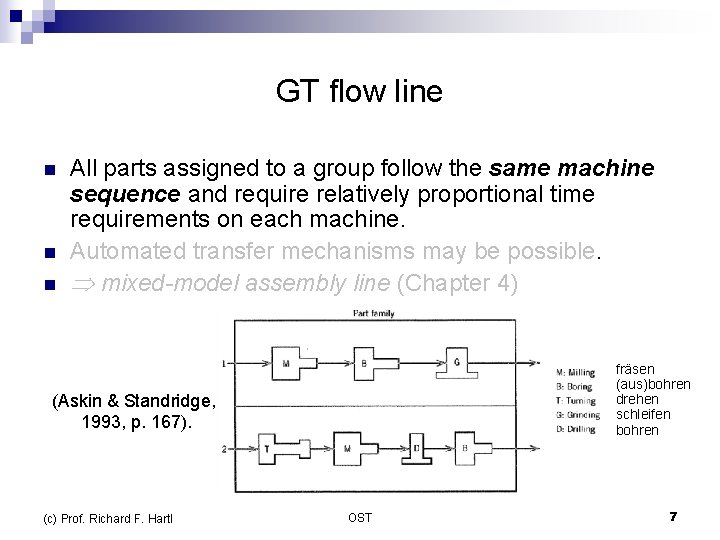
GT flow line n n n All parts assigned to a group follow the same machine sequence and require relatively proportional time requirements on each machine. Automated transfer mechanisms may be possible. mixed-model assembly line (Chapter 4) fräsen (aus)bohren drehen schleifen bohren (Askin & Standridge, 1993, p. 167). (c) Prof. Richard F. Hartl OST 7

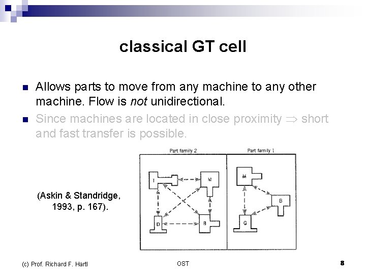
classical GT cell n n Allows parts to move from any machine to any other machine. Flow is not unidirectional. Since machines are located in close proximity short and fast transfer is possible. (Askin & Standridge, 1993, p. 167). (c) Prof. Richard F. Hartl OST 8

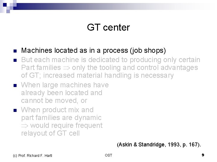
GT center n n Machines located as in a process (job shops) But each machine is dedicated to producing only certain Part families only the tooling and control advantages of GT; increased material handling is necessary When large machines have already been located and cannot be moved, or When product mix and part families are dynamic would require frequent relayout of GT cell (Askin & Standridge, 1993, p. 167). (c) Prof. Richard F. Hartl OST 9

Cellular manufacturing n n n n Group technology Parts with similar features are manufactured Small "focused factories" are created as independent operating units within large facilities. Divide the manufacturing facility into small groups Each cell is dedicated to a specified family or set of part types A cell is a small group of machines, tools, and handling equipment Since machines are located in close proximity short and fast transfer is possible (c) Prof. Richard F. Hartl OST 10

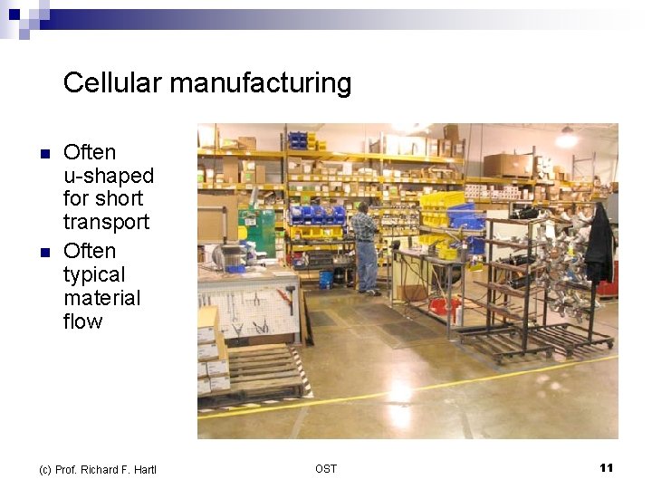
Cellular manufacturing n n Often u-shaped for short transport Often typical material flow (c) Prof. Richard F. Hartl OST 11

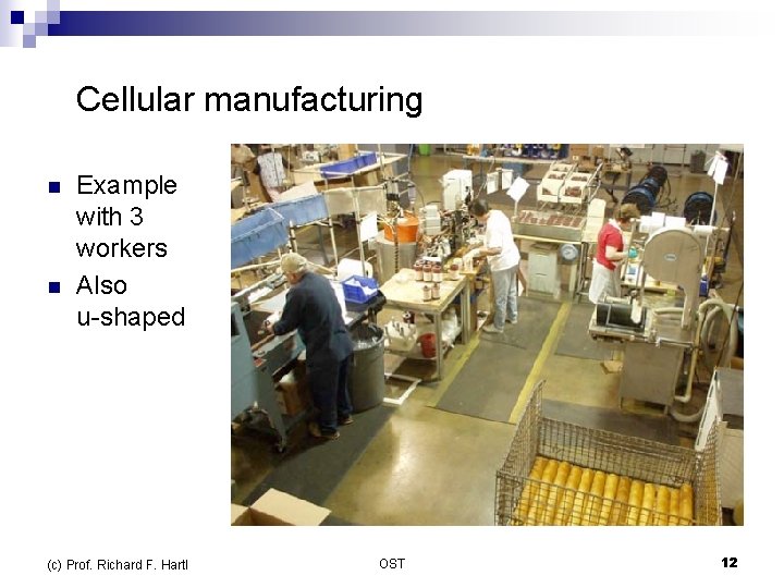
Cellular manufacturing n n Example with 3 workers Also u-shaped (c) Prof. Richard F. Hartl OST 12

Cellular manufacturing n Advantages: ¨ Short transportation and handling (usually within cell) ¨ Short setup times because often same tools and fixtures can be used (products are similar) ¨ High flexibility (quick reaction on changes) ¨ Clear arrangement, few tools/machines easy to control ¨ High motivation and satisfaction of workers (identification with “their" products) ¨ Small lot sizes possible ¨ Short flow times (c) Prof. Richard F. Hartl OST 13

Cellular manufacturing • How to build groups? – Similiar parts (similiar process flow/machine usage, same materials, …) are grouped – Visual inspection – Classification and coding based on design and production data (time consuming, no universally applicable system is available) – Production Flow Anlaysis (PFA), i. e. mathematical models (c) Prof. Richard F. Hartl OST Chapter 3 / 14

Production Flow Analysis Many clustering methods have been developed ¨ Can be classified into: ¨ n n n Part family grouping: Form part families and then group machines into cells Machine grouping: Form machine cells based upon similarities in part routing and then allocate parts to cells Machine-part grouping: Form part families and machine cells simultaneously (c) Prof. Richard F. Hartl OST 15

Machine-part grouping n Construct matrix of machine usage by parts n sort rows (machines) and columns (parts) so that a block -diagonal shape is obtained (c) Prof. Richard F. Hartl OST 16

Machine-part grouping n How can this sorting can be done systematically? ¨ Various heuristic and exact methods have been developed. The simplest one is binary ordering, also known as “rank order clustering” or “King’s algorithm“ (c) Prof. Richard F. Hartl OST 17

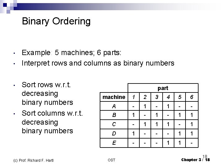
Binary Ordering • • Example: 5 machines; 6 parts: Interpret rows and columns as binary numbers Sort rows w. r. t. decreasing binary numbers Sort columns w. r. t. decreasing binary numbers (c) Prof. Richard F. Hartl part machine 1 2 3 4 5 6 A - 1 - - B 1 - 1 1 C - 1 1 1 - 1 D 1 - - - 1 1 E - - - 1 1 - OST 18 Chapter 3 / 18

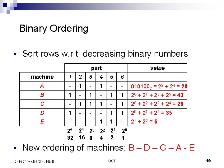
Binary Ordering § Sort rows w. r. t. decreasing binary numbers part value machine 1 2 3 4 5 6 A - 1 - - B 1 - 1 1 2 + 24 = 20 0101002 = 2 20 + 21 + 2 3 + 25 = 43 C - 1 1 1 - 1 20 + 22 + 2 3 + 24 = 29 D 1 - - - 1 1 20 + 21 + 2 5 = 35 E - - - 1 1 - 21 + 22 = 6 25 24 23 22 21 32 16 8 4 2 § 20 1 New ordering of machines: B – D – C – A - E (c) Prof. Richard F. Hartl OST 19

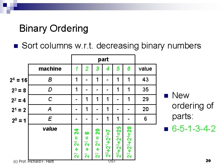
Binary Ordering n Sort columns w. r. t. decreasing binary numbers part 6 value 24 = 16 B 1 - 1 1 43 23 = 8 D 1 - - - 1 1 35 22 =4 C - 1 1 1 - 1 29 21 = 2 A - 1 - - 20 20 = 1 E - - - 1 1 - 6 value (c) Prof. Richard F. Hartl OST 22+23+24=28 5 20+23+24=25 4 20+21+22=7 3 22 + 24 = 20 2 21 + 22 = 6 1 23 + 24 = 24 machine n n New ordering of parts: 6 -5 -1 -3 -4 -2 20

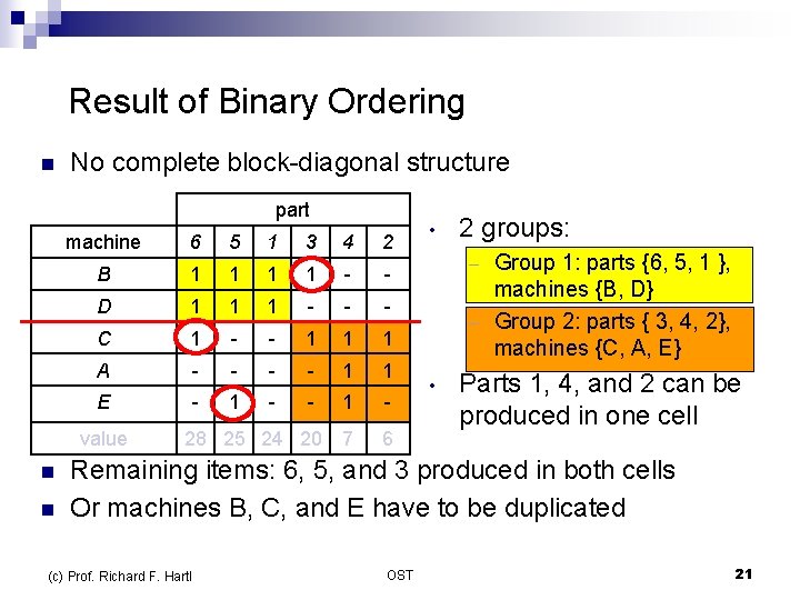
Result of Binary Ordering n No complete block-diagonal structure part machine 6 5 1 3 4 2 B 1 1 - - D 1 1 1 - - - C 1 - - 1 1 1 A - - 1 1 E - 1 - 7 6 value n n 28 25 24 20 • 2 groups: Group 1: parts {6, 5, 1 }, machines {B, D} – Group 2: parts { 3, 4, 2}, machines {C, A, E} – • Parts 1, 4, and 2 can be produced in one cell Remaining items: 6, 5, and 3 produced in both cells Or machines B, C, and E have to be duplicated (c) Prof. Richard F. Hartl OST 21

Repeated Binary Ordering n n Binary Ordering is a simple heuristic no guarantee that „optimal“ ordering is obtained Sometimes a better block-diagonal structure is obtained by repeatingthe Binary Ordering until there is no change anymore (c) Prof. Richard F. Hartl OST 22

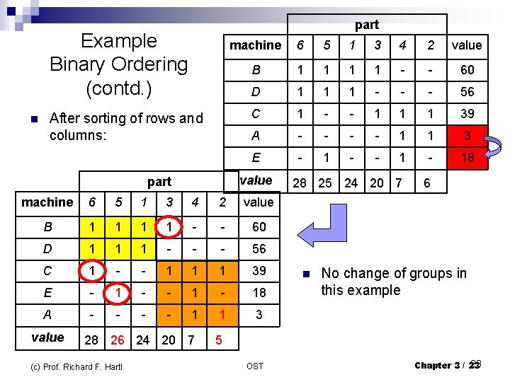
part Example Binary Ordering (contd. ) n After sorting of rows and columns: machine 6 5 1 3 4 2 value B 1 1 - - 60 D 1 1 1 - - - 56 C 1 - - 1 1 1 39 A - - 1 1 3 E - 1 - 18 28 25 24 20 7 6 value part machine 6 5 1 3 4 2 value B 1 1 - - 60 D 1 1 1 - - - 56 C 1 - - 1 1 1 39 E - 1 - 18 A - - 1 1 3 value 28 26 24 20 7 (c) Prof. Richard F. Hartl n No change of groups in this example 5 OST 23 Chapter 3 / 23

Single-Pass Heuristic • Considering capacities (Askin and Strandridge): • All parts must be processed in one cell (machines must be duplicated, if off-diagonal elements in matrix) All machines have capacities (normalized to be 1) Constraints on number of identical machines in a group Constraints on total number of machines in a group • • • (c) Prof. Richard F. Hartl OST 24

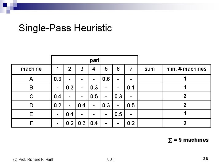
Single-Pass Heuristic - Example • • 7 parts, 6 machines Given matrix of processing times (incl. set up times) for typical lot size of parts on machines Entries in matrix not just 0/1 for used/not used) All times as percentage of total machine capacity • Maximal number of machines per cell: here at most 4 machines in a group • Not more than one machine of each type in a group (c) Prof. Richard F. Hartl OST 25

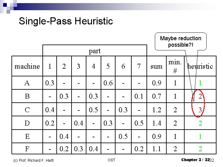
Single-Pass Heuristic part machine 1 2 3 4 5 6 7 sum min. # machines A 0. 3 - - - 0. 6 - - 0. 9 1 B - 0. 3 - - 0. 1 0. 7 1 C 0. 4 - - 0. 5 - 0. 3 - 1. 2 2 D 0. 2 - 0. 4 - 0. 3 - 0. 5 1. 4 2 E - 0. 4 - - - 0. 5 - 0. 9 1 F - 0. 2 0. 3 0. 4 - - 0. 2 1. 1 2 = 9 machines (c) Prof. Richard F. Hartl OST 26

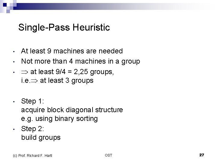
Single-Pass Heuristic • • • At least 9 machines are needed Not more than 4 machines in a group at least 9/4 = 2, 25 groups, i. e. at least 3 groups Step 1: acquire block diagonal structure e. g. using binary sorting Step 2: build groups (c) Prof. Richard F. Hartl OST 27

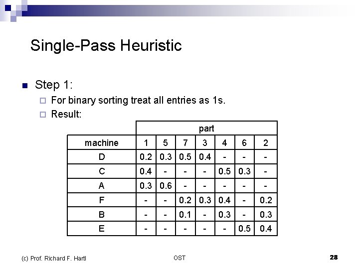
Single-Pass Heuristic n Step 1: For binary sorting treat all entries as 1 s. ¨ Result: ¨ part machine (c) Prof. Richard F. Hartl 1 5 7 3 D 0. 2 0. 3 0. 5 0. 4 C 0. 4 A 0. 3 0. 6 - - - 4 6 2 - - - 0. 5 0. 3 - - F - - 0. 2 0. 3 0. 4 - 0. 2 B - - 0. 1 - 0. 3 E - - - OST 0. 5 0. 4 28

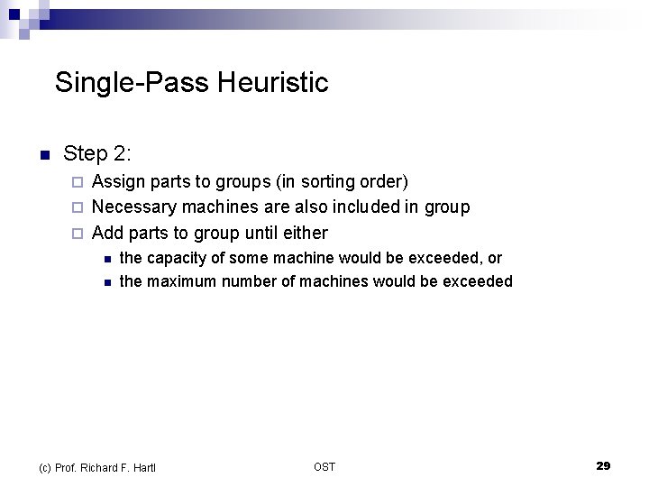
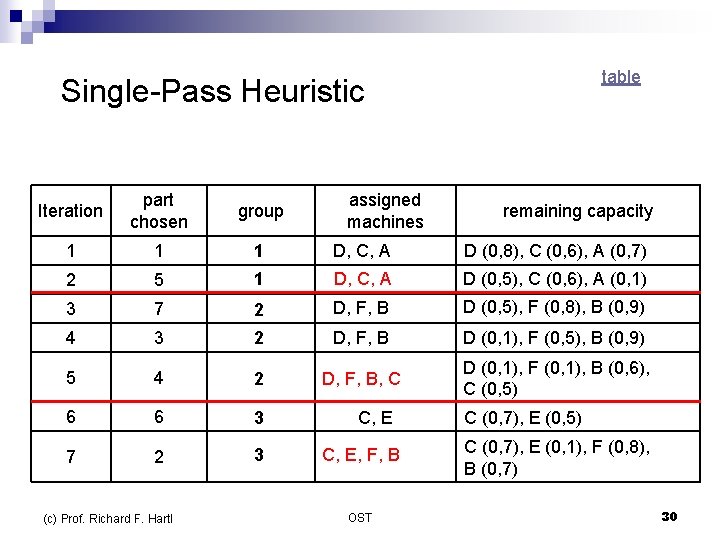
Single-Pass Heuristic n Step 2: Assign parts to groups (in sorting order) ¨ Necessary machines are also included in group ¨ Add parts to group until either ¨ n n the capacity of some machine would be exceeded, or the maximum number of machines would be exceeded (c) Prof. Richard F. Hartl OST 29

table Single-Pass Heuristic Iteration part chosen group 1 1 1 D, C, A D (0, 8), C (0, 6), A (0, 7) 2 5 1 D, C, A D (0, 5), C (0, 6), A (0, 1) 3 7 2 D, F, B D (0, 5), F (0, 8), B (0, 9) 4 3 2 D, F, B D (0, 1), F (0, 5), B (0, 9) 5 4 2 D, F, B, C D (0, 1), F (0, 1), B (0, 6), C (0, 5) 6 6 3 7 2 3 (c) Prof. Richard F. Hartl assigned machines C, E, F, B OST remaining capacity C (0, 7), E (0, 5) C (0, 7), E (0, 1), F (0, 8), B (0, 7) 30

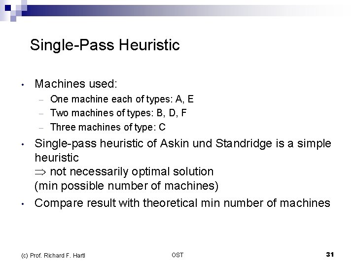
Single-Pass Heuristic • Machines used: One machine each of types: A, E – Two machines of types: B, D, F – Three machines of type: C – • • Single-pass heuristic of Askin und Standridge is a simple heuristic not necessarily optimal solution (min possible number of machines) Compare result with theoretical min number of machines (c) Prof. Richard F. Hartl OST 31

Single-Pass Heuristic part Maybe reduction possible? ! machine 1 2 3 4 5 6 7 min. sum heuristic # A 0. 3 - - - 0. 6 - - 0. 9 1 1 B - 0. 3 - - 0. 1 0. 7 1 2 C 0. 4 - - 0. 5 - 0. 3 - 1. 2 2 3 D 0. 2 - 0. 4 - 0. 3 - 0. 5 1. 4 2 2 E - 0. 4 - - - 0. 5 - 0. 9 1 1 F - 0. 2 0. 3 0. 4 - - 0. 2 1. 1 2 2 (c) Prof. Richard F. Hartl OST Chapter 3 / 3232

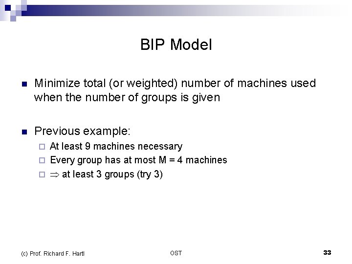
BIP Model n Minimize total (or weighted) number of machines used when the number of groups is given n Previous example: At least 9 machines necessary ¨ Every group has at most M = 4 machines ¨ at least 3 groups (try 3) ¨ (c) Prof. Richard F. Hartl OST 33

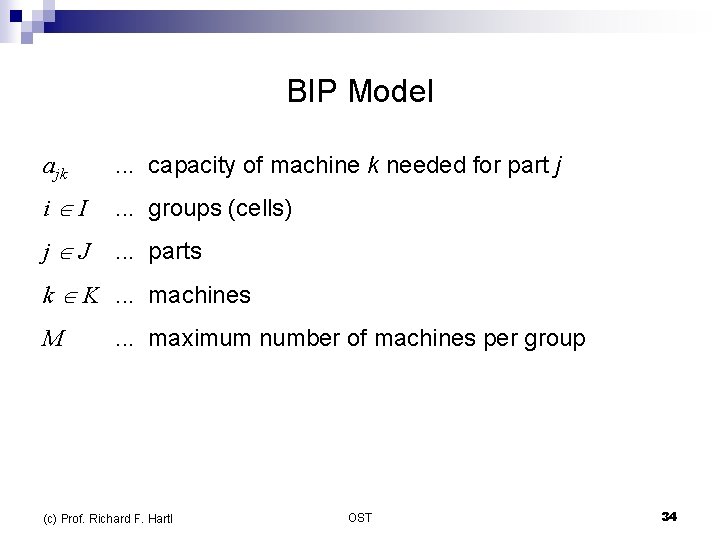
BIP Model ajk . . . capacity of machine k needed for part j i I . . . groups (cells) j J . . . parts k K. . . machines M . . . maximum number of machines per group (c) Prof. Richard F. Hartl OST 34

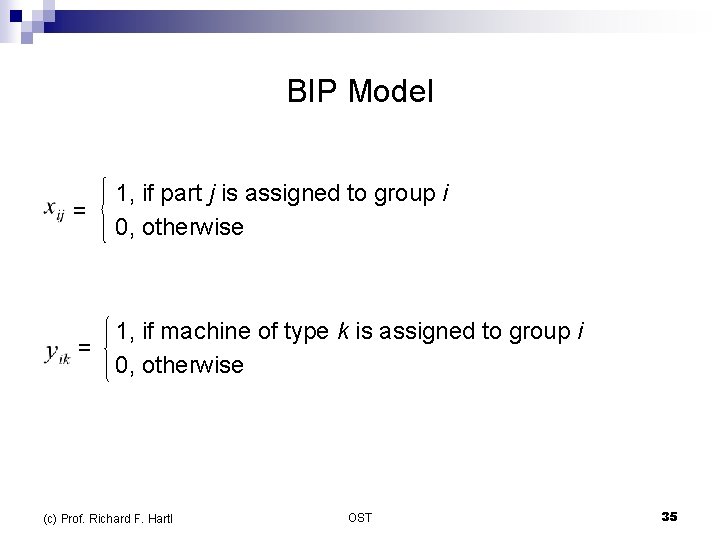
BIP Model = 1, if part j is assigned to group i 0, otherwise 1, if machine of type k is assigned to group i = 0, otherwise (c) Prof. Richard F. Hartl OST 35

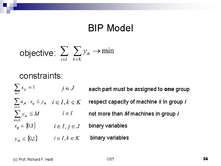
BIP Model objective: constraints: each part must be assigned to one group respect capacity of machine k in group i not more than M machines in group i binary variables (c) Prof. Richard F. Hartl OST 36

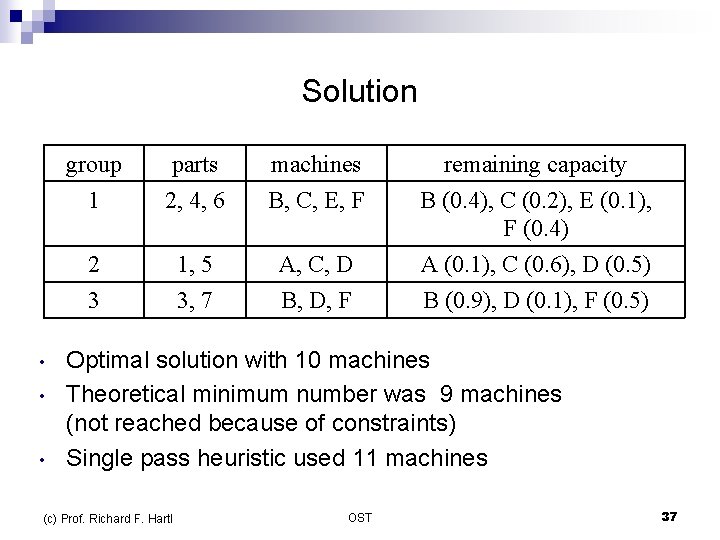
Solution • • • group 1 parts 2, 4, 6 machines B, C, E, F 2 3 1, 5 3, 7 A, C, D B, D, F remaining capacity B (0. 4), C (0. 2), E (0. 1), F (0. 4) A (0. 1), C (0. 6), D (0. 5) B (0. 9), D (0. 1), F (0. 5) Optimal solution with 10 machines Theoretical minimum number was 9 machines (not reached because of constraints) Single pass heuristic used 11 machines (c) Prof. Richard F. Hartl OST 37

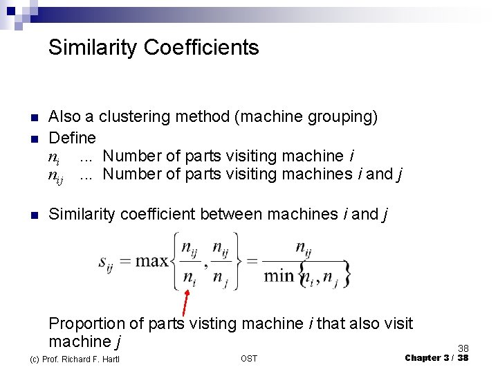
Similarity Coefficients n n n Also a clustering method (machine grouping) Define ni . . . Number of parts visiting machine i nij . . . Number of parts visiting machines i and j Similarity coefficient between machines i and j Proportion of parts visting machine i that also visit machine j (c) Prof. Richard F. Hartl OST 38 Chapter 3 / 38

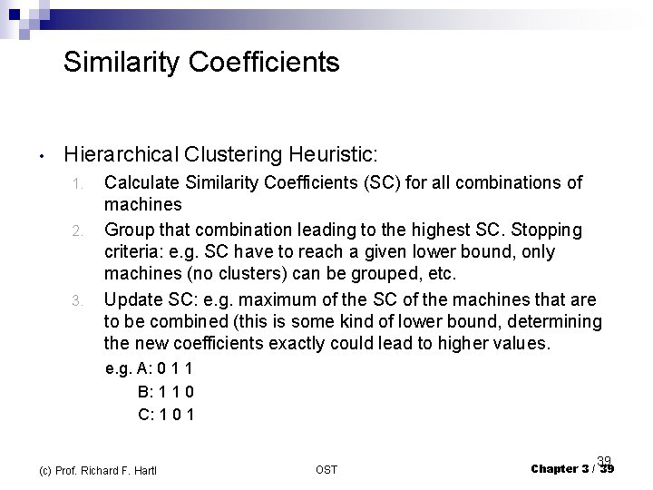
Similarity Coefficients • Hierarchical Clustering Heuristic: 1. 2. 3. Calculate Similarity Coefficients (SC) for all combinations of machines Group that combination leading to the highest SC. Stopping criteria: e. g. SC have to reach a given lower bound, only machines (no clusters) can be grouped, etc. Update SC: e. g. maximum of the SC of the machines that are to be combined (this is some kind of lower bound, determining the new coefficients exactly could lead to higher values. e. g. A: 0 1 1 B: 1 1 0 C: 1 0 1 (c) Prof. Richard F. Hartl OST 39 Chapter 3 / 39

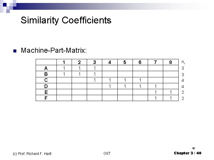
Similarity Coefficients n Machine-Part-Matrix: A B C D E F 1 1 1 2 1 1 3 1 1 1 4 1 1 5 1 1 6 1 1 7 1 1 1 8 1 1 ni 3 3 4 4 2 2 40 (c) Prof. Richard F. Hartl OST Chapter 3 / 40

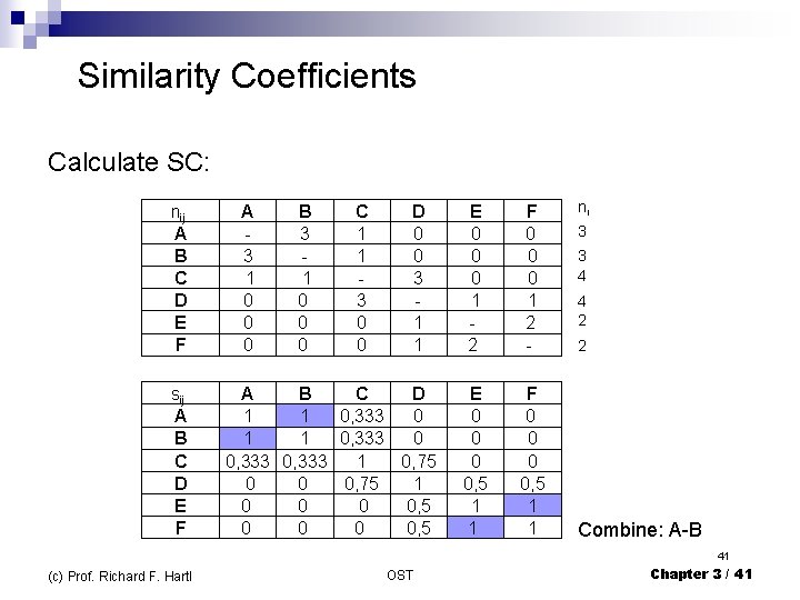
Similarity Coefficients Calculate SC: nij A B C D E F sij A B C D E F A 3 1 0 0 0 B 3 1 0 0 0 C 1 1 3 0 0 D 0 0 3 1 1 A B C D 1 1 0, 333 0 0, 333 1 0, 75 0 0 0, 75 1 0 0, 5 0 0, 5 E 0 0 0 1 - 2 F 0 0 0 1 2 - E 0 0, 5 1 1 F 0 0, 5 1 1 ni 3 3 4 4 2 2 Combine: A-B 41 (c) Prof. Richard F. Hartl OST Chapter 3 / 41

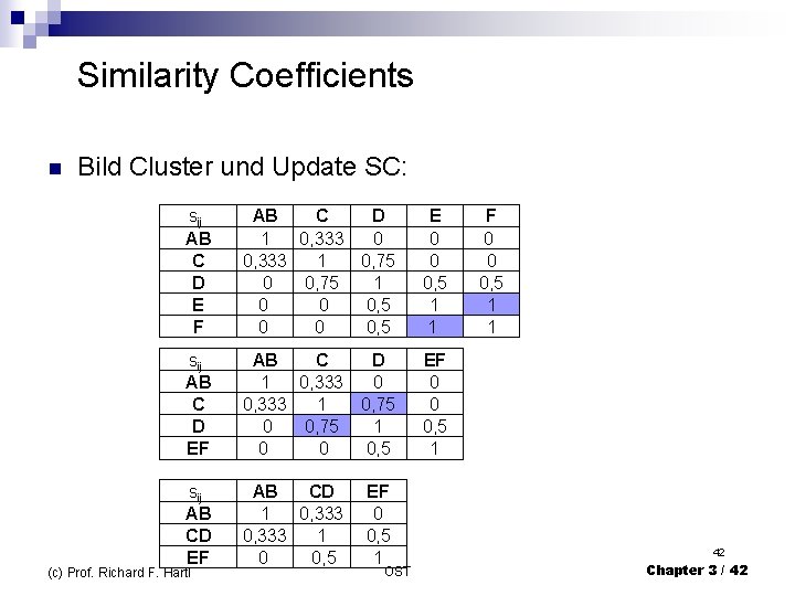
Similarity Coefficients n Bild Cluster und Update SC: sij AB C D E F AB C D 1 0, 333 0 0, 333 1 0, 75 0 0, 75 1 0 0 0, 5 0 0 0, 5 E 0 0 0, 5 1 1 sij AB C D EF AB C D 1 0, 333 0 0, 333 1 0, 75 0 0, 75 1 0 0 0, 5 EF 0 0 0, 5 1 sij AB CD EF AB CD 1 0, 333 1 0 0, 5 (c) Prof. Richard F. Hartl EF 0 0, 5 1 OST F 0 0 0, 5 1 1 42 Chapter 3 / 42

Similarity Coefficients n Dendogram: ¨ Graphical illustrations of possible groupings per threshold 43 (c) Prof. Richard F. Hartl OST Chapter 3 / 43

Graph Partitioning n n n Machines with common parts should be in same group Graph illustrating common parts Group forming can be seen as special case of graph partitioning (c) Prof. Richard F. Hartl OST Chapter 3 / 44

Graph Partitioning n n Given a graph with nodes and edges, find a partitioning of the node set into a (given) number of disjoint subsets of approximately equal size, such that the total cost of edges that connect nodes of different subsets is minimized. NP-hard optomization problem Various methods have been developed Simple and well-known heuristic by Kernighan and Lin (c) Prof. Richard F. Hartl OST Chapter 3 / 45

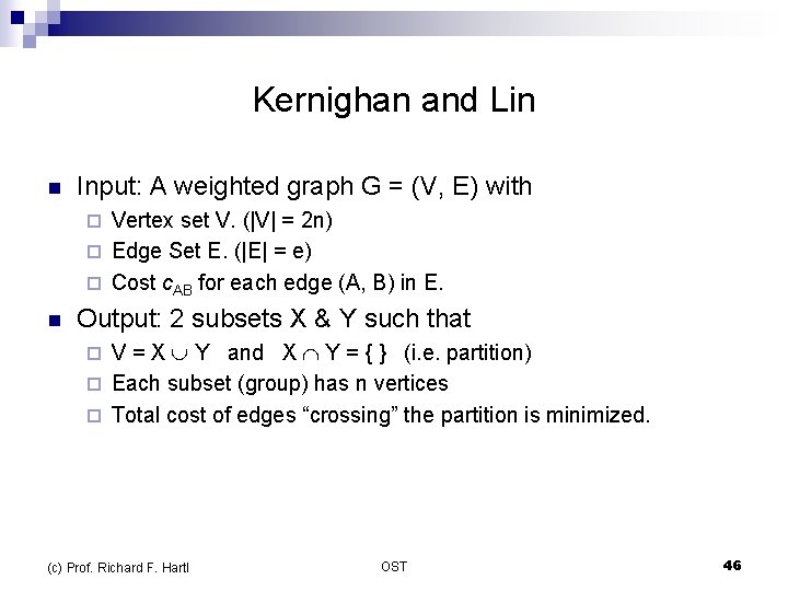
Kernighan and Lin n Input: A weighted graph G = (V, E) with Vertex set V. (|V| = 2 n) ¨ Edge Set E. (|E| = e) ¨ Cost c. AB for each edge (A, B) in E. ¨ n Output: 2 subsets X & Y such that V = X Y and X Y = { } (i. e. partition) ¨ Each subset (group) has n vertices ¨ Total cost of edges “crossing” the partition is minimized. ¨ (c) Prof. Richard F. Hartl OST 46

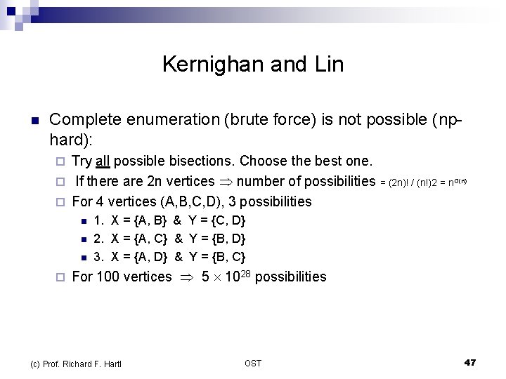
Kernighan and Lin n Complete enumeration (brute force) is not possible (nphard): Try all possible bisections. Choose the best one. ¨ If there are 2 n vertices number of possibilities = (2 n)! / (n!)2 = n. O(n) ¨ For 4 vertices (A, B, C, D), 3 possibilities ¨ n n n ¨ 1. X = {A, B} & Y = {C, D} 2. X = {A, C} & Y = {B, D} 3. X = {A, D} & Y = {B, C} For 100 vertices 5 1028 possibilities (c) Prof. Richard F. Hartl OST 47

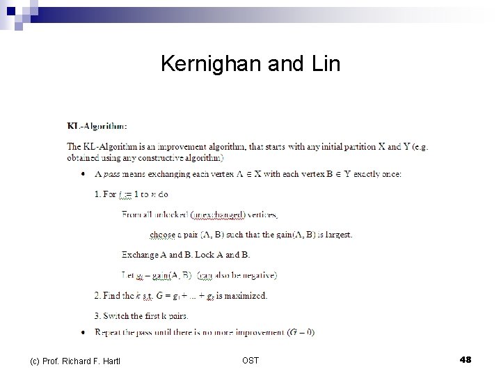
Kernighan and Lin (c) Prof. Richard F. Hartl OST 48

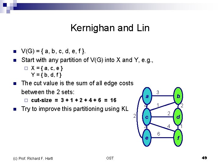
Kernighan and Lin n n V(G) = { a, b, c, d, e, f }. Start with any partition of V(G) into X and Y, e. g. , ¨ n The cut value is the sum of all edge costs between the 2 sets: ¨ n X = { a, c, e } Y = { b, d, f } cut-size = 3 + 1 + 2 + 4 + 6 = 16 a 4 Try to improve this partitioning using KL 2 3 1 OST d 4 3 (c) Prof. Richard F. Hartl 2 2 c e b 6 1 f 49

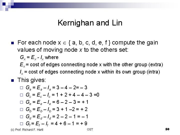
Kernighan and Lin n For each node x { a, b, c, d, e, f } compute the gain values of moving node x to the others set: Gx = Ex - Ix where Ex = cost of edges connecting node x with the other group (extra) Ix = cost of edges connecting node x within its own group (intra) n This gives: ¨ ¨ ¨ Ga = Ea – Ia = 3 – 4 – 2= – 3 Gc = Ec – Ic = 1 + 2 + 4 – 3 =0 Ge = Ee – Ie = 6 – 2 – 3 = + 1 Gb = Eb – Ib = 3 + 1 – 2 = + 2 Gd = Ed – Id = 2 – 1 = – 1 Gf = Ef – If = 4 + 6 – 1 = + 9 (c) Prof. Richard F. Hartl OST 50

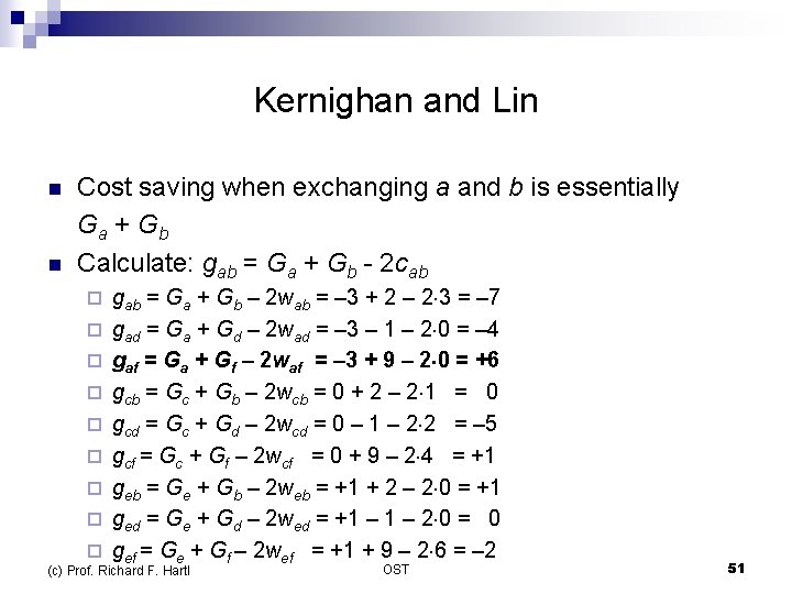
Kernighan and Lin n n Cost saving when exchanging a and b is essentially Ga + Gb Calculate: gab = Ga + Gb - 2 cab ¨ ¨ ¨ ¨ ¨ gab = Ga + Gb – 2 wab = – 3 + 2 – 2 3 = – 7 gad = Ga + Gd – 2 wad = – 3 – 1 – 2 0 = – 4 gaf = Ga + Gf – 2 waf = – 3 + 9 – 2 0 = +6 gcb = Gc + Gb – 2 wcb = 0 + 2 – 2 1 = 0 gcd = Gc + Gd – 2 wcd = 0 – 1 – 2 2 = – 5 gcf = Gc + Gf – 2 wcf = 0 + 9 – 2 4 = +1 geb = Ge + Gb – 2 web = +1 + 2 – 2 0 = +1 ged = Ge + Gd – 2 wed = +1 – 2 0 = 0 gef = Ge + Gf – 2 wef = +1 + 9 – 2 6 = – 2 (c) Prof. Richard F. Hartl OST 51

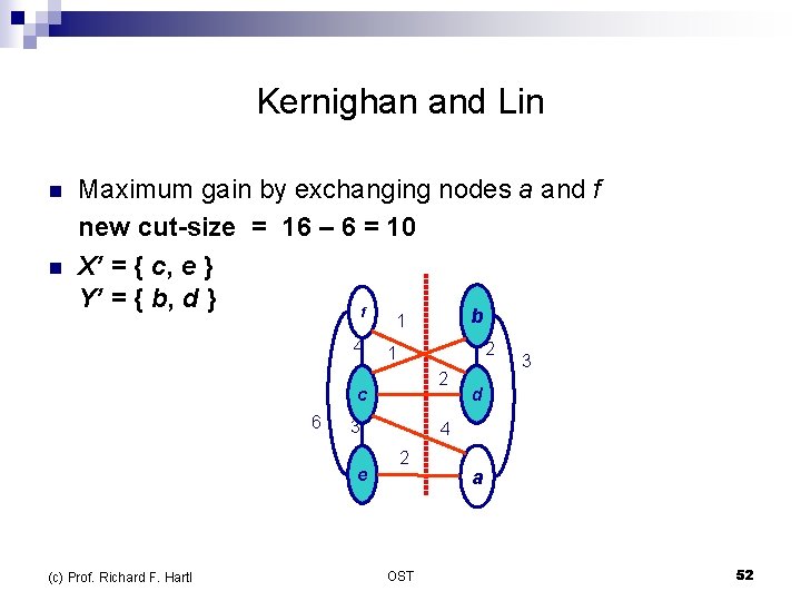
Kernighan and Lin n n Maximum gain by exchanging nodes a and f new cut-size = 16 – 6 = 10 X’ = { c, e } Y’ = { b, d } f b 1 4 2 1 2 c 6 3 e (c) Prof. Richard F. Hartl 3 d 4 2 OST a 52

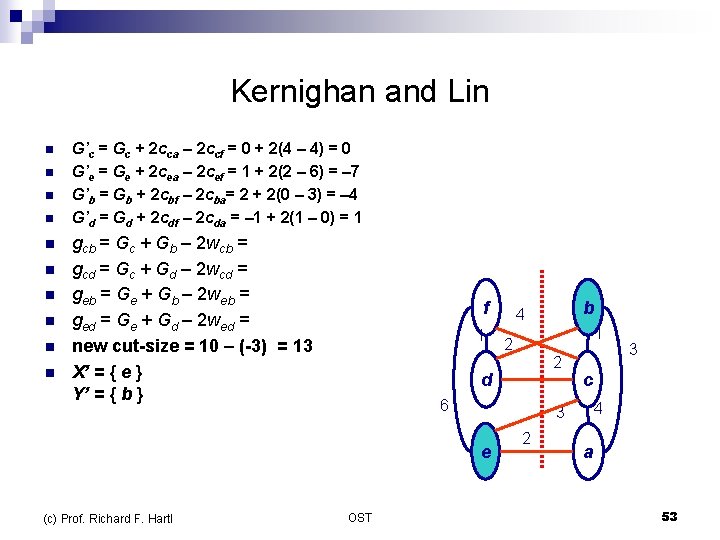
Kernighan and Lin n n G’c = Gc + 2 cca – 2 ccf = 0 + 2(4 – 4) = 0 G’e = Ge + 2 cea – 2 cef = 1 + 2(2 – 6) = – 7 G’b = Gb + 2 cbf – 2 cba= 2 + 2(0 – 3) = – 4 G’d = Gd + 2 cdf – 2 cda = – 1 + 2(1 – 0) = 1 gcb = Gc + Gb – 2 wcb = gcd = Gc + Gd – 2 wcd = geb = Ge + Gb – 2 web = ged = Ge + Gd – 2 wed = new cut-size = 10 – (-3) = 13 X’ = { e } Y’ = { b } f 1 1 2 2 d 6 OST 2 3 c 4 3 e (c) Prof. Richard F. Hartl b 4 a 53

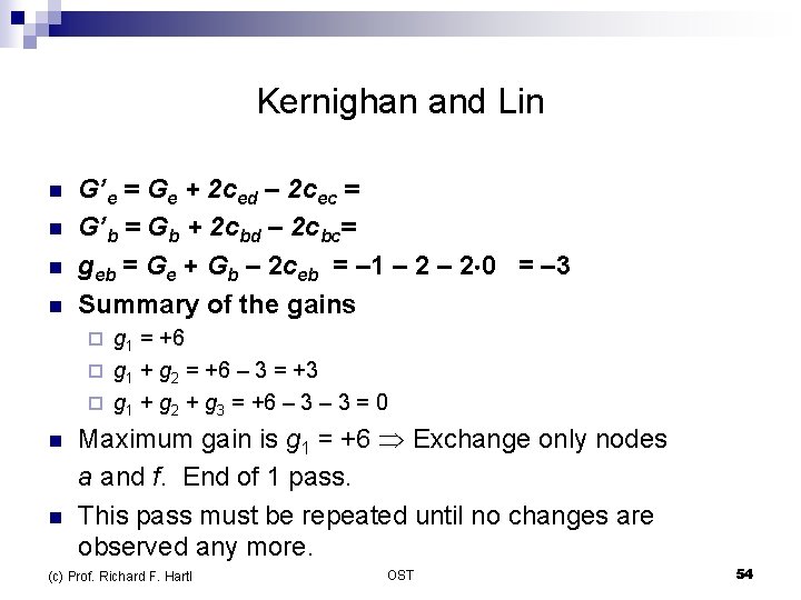
Kernighan and Lin n n G’e = Ge + 2 ced – 2 cec = G’b = Gb + 2 cbd – 2 cbc= geb = Ge + Gb – 2 ceb = – 1 – 2 0 = – 3 Summary of the gains g 1 = +6 ¨ g 1 + g 2 = +6 – 3 = +3 ¨ g 1 + g 2 + g 3 = +6 – 3 = 0 ¨ n n Maximum gain is g 1 = +6 Exchange only nodes a and f. End of 1 pass. This pass must be repeated until no changes are observed any more. (c) Prof. Richard F. Hartl OST 54

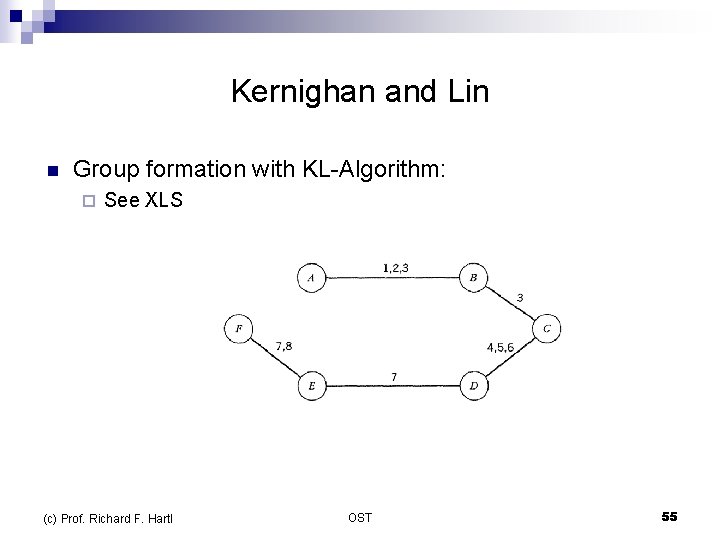
Kernighan and Lin n Group formation with KL-Algorithm: ¨ See XLS (c) Prof. Richard F. Hartl OST 55

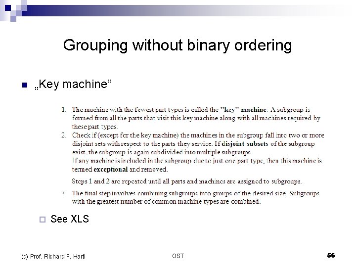
Grouping without binary ordering n „Key machine“ ¨ See XLS (c) Prof. Richard F. Hartl OST 56