Noiseless Coding Introduction n Noiseless Coding Compression without

Noiseless Coding

Introduction n Noiseless Coding Compression without distortion n Basic Concept Symbols with lower probabilities are represented by the binary indices with longer length n Methods Huffman codes, Lempel-Ziv codes, Arithmetic codes and Golomb codes

Entropy n Consider a set of symbols S={S 1, . . . , SN}. n The entropy of the symbols is defined as where P(Si) is the probability of Si.

Example: Consider a set of symbols {a, b, c} with P(a)=1/4, P(b)=1/4 and P(c)=1/2. The entropy of the symbols is then given by

Consider a message containing symbols in S. Define rate of a source coding technique as the average number of bits representing each symbol after compressing.

Example: Suppose the following message is desired to be compressed. a a a b c a Suppose a encoding technique uses 7 bits to represent the message. The rate of the encoding technique therefore is 7/6. (since there are 6 symbols)

Shannon’s source coding theorem: The lowest rate for encoding a message without distortion is the entropy of the symbols in the message.

Therefore, in an optimal noiseless source encoder, the average number of bits used to represent each symbol Si is It will take larger number of bits to represent a symbol having small probability.

Because the entropy is the limit of the noiseless encoder, we usually call the noiseless encoder, the entropy encoder.

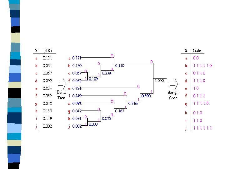
Huffman Codes n We start with a set of symbols , where each symbol is associated with a probability. n Merge two symbols having lowest probabilities to a new symbol.

n Repeat the merging process until all the symbols are merged to a single symbol. n Following the merging path, we can form the Huffman codes.

Example n Consider the following three symbols : a ( with prob. 0. 5 ) b ( with prob. 0. 3 ) c ( with prob. 0. 2 )

Merging Process 1 a b c 1 0 0 Huffman Codes : a b c 1 01 00

Example n Suppose the following message is desired to be compressed. a a a b c a n The results of the Huffman coding are : 1 1 1 01 00 1 n Total # of bits used to represent the message : 8 bits (Rate=8/6=4/3)

n If the message is not compressed by the Huffman codes , each symbol should be represented by 2 bits. Total # of bits used to represent the message therefore is 12 bits. n We have saved 4 bits using the Huffman codes.

Example

Discussions n It does not matter how the symbols are arranged. n It does not matter how the final code tree are labeled (with 0 s and 1 s). n Huffman code is not unique.

Lempel-Ziv Codes n Parse the input sequence into nonoverlapping blocks of different lengths. n Construct a dictionary based on the blocks. n Use the dictionary for both encoding and decoding.

n It is NOT necessary to pre-specify the probability associated with each symbol.

Dictionary Generation process 1. 2. 3. 4. 5. Initialize the dictionary to contain all blocks of length one. Search for the longest block W which has appeared in the dictionary. Encode W by its index in the dictionary. Add W followed by the first symbol of the next block to the dictionary. Go to Step 2.

Example n Consider the following input message abaaba n Initial dictionary: index entry 0 a 1 b

encoder side n. W = a, output 0 n Add ab to the dictionary index 0 1 2 entry a b ab abaaba

encoder side n. W = b, output 1 n Add ba to the dictionary index 0 1 2 entry a b ab 3 ba abaaba

encoder side n. W = a, output 0 n Add aa to the dictionary index 0 1 2 entry a b ab 3 4 ba aa abaaba

encoder side n. W = ab, output 2 n Add aba to the dictionary index 0 1 2 entry a b ab 3 4 5 ba aa abaaba

encoder side n. W = a, output 0 n Stop index 0 1 2 entry a b ab 3 4 5 ba aa abaaba

decoder side n Initial dictionary 0 index entry 0 a 1 b n Input 0, generate a a

decoder side n Receive 1, generate b n Add ab to the dictionary 1 a b index 0 1 2 entry a b ab

decoder side n Receive 0, generate a n Add ba to the dictionary 0 a b a index 0 1 2 entry a b ab 3 ba

decoder side n Receive 2, generate ab n Add aa to the dictionary index 0 1 2 entry a b ab 3 4 ba aa 2 a b a a b

decoder side n Receive 0, generate a n Add aba to the dictionary index 0 1 2 entry a b ab 3 4 5 ba aa aba 0 a b a

Example

Example Consider again the following message a a a b c The initial dictionary is given by index 0 1 2 entry a b c a

After the encoding process, the output of the encoder is given by 0 3 1 2 0 The final dictionary is given by index 0 1 2 entry a b c 3 4 5 6 aa aab bc ca

decoder side n Initial dictionary 0 index 0 1 2 entry a b c n Receive 0, generate a a

decoder side n Receive 3, generate ? n Decoder get stuck !!! index 0 1 2 n We entry a b c 3 a ? need Welch correction to this problem.

Welch correction It turns out that this behavior can arise whenever one sees a pattern of the form xwxwx where x is a single symbol, and w is either empty or a sequence of symbols such that xw already appears in the encoder and decoder table, but xwx does not.

Welch correction In this case the encoder will send the index for xw, and add xwx to the table with a new index i. Next it will parse xwx and send the new index i. The decoder will receive the index i but will not yet have the corresponding word in the dictionary.

Welch correction Therefore, when the decoder can not find the corresponding word for an index i, the word must be xwx, where xw can be found from the last decoded symbols.

decoder side Here, the last decoded symbol is a. Therefore, x=a, and w= , Hence, xwx=aa. index 0 1 2 entry a b c 3 aa 3 a a a

decoder side n Receive 1, generate b n Add aab to the dictionary index 0 1 2 entry a b c 3 4 aa aab 1 a a a b

decoder side n Receive 2 and 0, generate c and a n Final dictionary index 0 1 2 entry a b c 3 4 5 6 aa aab bc ca 2 0 a a a b c a

Example Consider the following message abababa After the encoding process, the output of the encoder is given by 0124 The final dictionary is given by index entry 0 a 1 b 2 ab 3 ba 4 aba

decoder side n Receive 0, 1 and 2, generate a, b and ab n current dictionary index entry 0 a 1 b 2 ab 3 ba 0 1 2 a b

decoder side n Receive 4, generate ? n current dictionary index entry 0 a 1 b 2 ab 3 ba 4 a b ?

Here, the last decoded symbol is ab. Therefore, x=a, and w= b, Hence, xwx=aba. index entry 0 a 1 b 2 ab 3 ba 4 a b a b a

Discussions n Theoretically, the size of the dictionary can grow infinitely large. n In practice, the dictionary size is limited. Once the limit is reached, no more entries are added. Welch had recommended a dictionary of size 4096. This corresponds to 12 bits per index.

Discussions n The length of indices may vary. When the number of entries n in the dictionary is such that 2 m n > 2 m-1 then the length of indices can be m.

Discussions n Use the message a a a b c a as an example, the encoded indices are 0 3 00 1 001 2 11 010 Need 13 bits (Rate=13/6) 0 000

Discussions The above examples, as most other illustrative examples in the literature, does not result in real compression. Actually, more bits are used to represent the indices than the original data. This is because the length of the input data in the example is too short. n In practice, the Lempel-Ziv algorithm works well (lead to actual compression) only when the input data is sufficiently large and there are sufficient redundancy in the data. n

Discussions n Many popular programs (e. g. Unix compress and uncompress, gzip and gunzip, GIF format and Windows Win. Zip) are based on the Lempel-Ziv algorithm.

Arithmetic Codes n. A message is represented by an interval of real numbers between 0 and 1. n As the message becomes longer , the interval needed to represent it becomes smaller. =>The number of bits needed to specify that interval grows.

Arithmetic Codes n Successive symbols of the message reduce the size of the interval according to the symbol probabilities.

Example n Again we consider the following three symbols : a ( with prob. 0. 5 ) b ( with prob. 0. 3 ) c ( with prob. 0. 2 ) n Suppose we also encode the same message as the previous example : a a a b c a

The encoding process 1 0. 5 0. 25 c 0. 125 0. 1 0. 25 0. 125 0. 09625 0. 0925 b 0. 5 0. 1 0. 09625 0. 0625 a 0 0 0. 0625 0. 0925 a a a b c a Final interval

Final interval n The final interval therefore is [ 0. 0625 , 0. 09625 ) n Any number in this final interval can be used for the decoding process. n For instance , we pick 0. 09375 ∈ [ 0. 0625 , 0. 09625 )

1 0. 5 0. 25 c 0. 125 0. 1 0. 0925 b 0. 25 0. 125 0. 09625 0. 0625 a 0 0 0. 09375 ∈ [ 0, 0. 5 ) output 0 0. 09375 ∈ [ 0, 0. 125 ) a output a 0. 09375 ∈ [ 0, 0. 25 ) output 0 a 0. 0625 0. 09375 ∈ [ 0. 925, 0. 1 ) output c 0. 09375 ∈ [ 0. 0625, 0. 1 ) output b 0. 0925 0. 09375 ∈ [ 0. 0925, 0. 09625 ) output a

Decoder Therefore , the decoder successfully identify the source sequence a a a b c a n Note that 0. 09375 can be represented by the binary sequence 0 0 0 1 1 n (0. 5) (0. 25) (0. 125) (0. 0625) (0. 03125) n We only need 5 bits to represent the message (Rate=5/6).

Discussions n Given the same message a a a b c a n No compression 12 bits n Huffman codes 8 bits n Lempel-Ziv 13 bits n Arithmetic codes 5 bits

Discussions n The length of the interval may become very small for a long message, causing underflow problem.

Discussions n The encoder does not transmit any thing until the entire message has been encoded. In most applications an incremental mode is necessary.

Discussions n The symbol frequencies (i. e. , probabilities) might vary with time. It is therefore desired to use an adaptive symbol frequency model for encoding and decoding.

Golomb Codes n Well-suited for messages containing lots of 0’s and not too many 1’s. n Example: Fax Documents

n First step of Golomb Code: Convert the input sequence into integers n Example: – 0010000000001000000000001 – 2, 6, 9, 10, 27

n Second step of Golomb code: Convert the integers into encoded bitstream – Select an integer m. – For each integer obtained from the first step n, compute q and r, where n=qm+r

– Binary code for n has two parts: 1. q is coded in unary 2. r can be coded in fixed length code or variable length code. – Example: m=5, value of r can be 0, 1, 2, 3, 4. Their VLC (denoted by )are:

– Example: The binary code for n has the following form: Therefore, the encoded bistream is given by

n References 1. K. Sayood, Introduction to Data Compression, Morgan Kaufmann, 2000.