Multigrid Methods for Solving the Convection Diffusion Equations

Multigrid Methods for Solving the Convection -Diffusion Equations Chin-Tien Wu National Center for Theoretical Sciences Mathematics Division Tsing-Hua University

Motivation 1. Incompressible Navier-Stokes equation models many flows in practices. Linearized backward Euler Oseen Problem Discretization Saddle Point Problem

2. A preconditioning technique proposed by Silvester, Elman, Kay and Wathen for solving linearized incompressible Naiver-Stokes has been shown to be very efficient. (J. Comput. and Appl. Math. 2001 No 128 P. 261 -279). 3. For achieving efficiency, a robust Poisson solver and a scalar convection-diffusion solver are needed. 4. Mulrigrid is efficient for solving Poisson problem. Can we have a robust multigrid solver for the convection-diffusion problems?

Convection-Diffusion Equation The problem we consider here is where sufficiently smooth. for some constant c 0 and b, c and f are

Challenges in solving the convection-diffusion problem 1. When the convection is dominant, <<1, the solution has sharp gradients due to the presents of Dirichlet outflow boundaries or discontinuity in inflow boundaries. 2. The associated linear system is not symmetric. What are the foundations for building an efficient and accurate solver? I. III. IV. Stable discretization methods for FEM. A good mesh. Reliable error estimation. Fast iterative linear solver.

I. Discretization • Galerkin FEM • Streamline diffusion upwinding FEM by Hughes and Brooks 1979 • Discontinuous Galerkin FEM by Reed and Hill 1973 • Edge-averaged FEM by Xu and Zikatanov 1999 (the linear system form this discretization is an M-matrix)

Example 1: Characteristic and downstream layers 1 1 1 0 Solution from Galerkin discretization on 32 x 32 grid . 1 Solution from SDFEM discretization on 32 x 32 grid

II. Methods for producing a good mesh? 1. Delaunay triangulation (DT): DT maximizes the minimal angle of the triangulation. 2. Advancing Front algorithm (AF): controls the element shape through control variables such as element stretch ratio (by Löhner 1988). 3. Advancing front Delaunay triangulation: combination of DT and AF (by Mavriplis 1993, Müller 1993 and Marcum 1995). 4. Longest side bisection: produces nested grids and guarantee the minimal angle on the fine grid is greater than or equal to half of the minimal angle on the coarse grid (by Rivara 1984). 5. Mesh relaxation includes moving mesh by equidistribution, MMPDE (by Huang, Ren and Russell 1994), and moving mesh FEM (by Carlson and Miller 1994, and Baines 1994).

III. A posteriori error indicators are used to pinpoint where the errors are large. • A posteriori error estimation based on residual is proposed by Babuška and Rheinboldt 1978 • A posteriori error estimation based on solving a local problem is proposed by Bank and Weiser 1985 • A posteriori error estimation based on recovered gradient is proposed by Zienkiewicz and Zhu 1987 • A posteriori error estimations for the convection-diffusion problems are proposed by Verfürth 1998, Kay and Silvester 2001.

Adaptive Solution Strategies Strategy I : i Solve Compute error indicator Refine mesh ii i (Kay and Silvester 2001) ii In mesh refinement, we employee the maximum marking strategy:

Improve Solution Accuracy by Mesh Refinement Problem 1: Adaptive meshes with threshold 0. 01 in the maximum marking strategy Contour plots of solutions on adaptive meshes

IV. Solving Linear System Ax=b by Iterative Methods: • Stationary Methods: Jacobi, Gauss Seidel (GS), SOR. • Krylov Subspace Methods: GMRES, by Saad and Schultz 1986, and MINRES, by Paige and Saunders 1975. • Multigrid Methods: Geometric multigrid (MG), by Fedorenko 1961, and algebraic multigrid (AMG), by Ruge and Stüben 1985. Why Multigrid? Numerical Scheme Operations for Square/Cube 2 -D 3 -D Gaussian elimination O(N 2) O(N 7/3) Jacobi O(N 2) O(N 5/3) Conjugate Gradient O(N 3/2) O(N 4/3) Multigrid O(Nlog(N)) Multigrid convergence is independent with problem size.

Why multigrid works? 1. Relaxation methods converge slowly but smooth the error quickly. Consider Richardson relaxation: Fourier analysis shows that , after m relaxation and choosing 2. Smooth error modes are more oscillatory on coarse grids. Smooth errors can be better corrected by relaxation on coarser grids.

Multigrid (I) Multigrid (MG) Algorithm: MG Error reduction operator: Pre-smoothing only Post-smoothing only

Restriction Prolongation MG V-cycle AMG Coarsening Adaptive refinement Multigrid (II)

Multigrid (GMG) and Algebraic Multigrid (AMG) MG AMG 1. A priori generated coarse grids are needed. Coarse grids need to be generated based on geometric information of the domain. 1. A priori generated coarse grids are not needed! Coarse grids are generated by algebraic coarsening from matrix on fine grid. 2. Interpolation operators are defined 2. independent with coarsening process. Interpolation operators are defined dynamically in coarsening process. 3. Smoother is not always fixed. 3. Smoother is fixed.

Multigrid Components Prolongation Restriction GMG : linear interpolation AMG R/S coarsening Coarse grid operator Discretization on VH • Smoothing operator Es: 21 22 23 24 25 16 17 18 19 20 11 12 13 14 15 6 7 8 9 10 1 2 3 4 5 Backward H-line GS Forward V-line GS 21 22 23 24 25 16 17 18 19 20 11 12 13 14 15 6 7 8 9 10 1 2 3 4 5 Backward V-line GS

GMG Convergence Smoothing property: Approximation property: Choices of interploations: • Linear interpolation: • Operator-dependent interpolation: De Zeeuw 1990 Recent results: Convergence needs robust smoothers together with semi-coarsening and operator dependent prolongation for the convection-diffusion equation (Reusken 2002).

GMG Convergence for Problem 1 Auxiliary inequalities: 1. 2. Theorem 1: Horizontal line Gauss-Seidel (HGS) converges for Theorem 2. : Geometric multigrid with HGS smoother and bilinear interpolation converge and mesh 16 x 16 10 -2 10 -3 10 -4 10 -5 mesh 6 7 4 5 3 4 16 x 16 32 x 32 8 8 64 x 64 9 8 6 4 HGS convergence on rectangular mesh 10 -2 10 -3 10 -4 10 -5 32 x 32 4 4 2 3 2 2 1 1 64 x 64 5 4 2 2 MG convergence on rectangular mesh

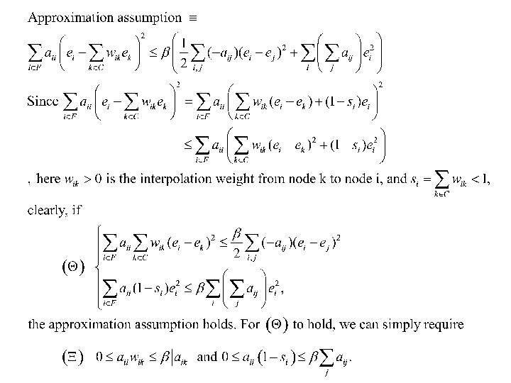
AMG convergence Smoothing assumption: Approximation assumption: AMG works when A is a symmetric positive definite M-matrix.

• Smooth error is characterized by • Smoother errors vary slowly in the direction of strong connection, from ei to ej , where are large. • AMG coarsening should be done in the direction of the strong connections. • In the coarsening process, interpolation weights are computed so that the approximation assumption is satisfied. (detail see Ruge and Stüben 1985)

AMG works for Problem 1 Assuming the Galerkin coarse grid correction satisfied the approximation property, inequalities in the auxiliary lemmas and the approximation assumption imply • AMG converges more rapidly than GMG as long as Smooth error es satisfies Smooth error varies slowly along strong connected direction when h>> 2/3. • R/S AMG coarsening and interpolation work.

AMG Coarsening Algorithm (I)

AMG Coarsening Algorithm (II)

AMG Coarsening SDFEM discretization of Problem 1 with has matrix stencil: C-point AMG coarsening with strong connection parameter /h << 0. 25 C-point

AMG Coarsening on Uniform Meshes Problem 1: b=(0, 1) Flow field Coarse grids from GMG coarsening Coarse grids from AMG coarsening

Problem 2: circulating flow b=(2 y(1 -x 2), 2 x(1 -y 2)) Flow field Coarse grids from GMG coarsening Coarse grids from AMG coarsening

GMG and AMG as a Solver (I) Problem 1: On the uniform mesh: level GMG AMG 3 13 7 3 27 8 3 51 11 2 13 6 2 26 7 2 35 8 1 12 6 1 16 6 1 17 6 =10 -3 -2 On the adaptive mesh: =10 -4 Level GMG AMG 4 9 6 4 22 8 4 59 14 3 8 8 3 24 9 3 57 10 2 7 6 2 18 8 2 47 8 1 7 5 1 17 7 1 34 7 =10 -4

GMG and AMG as a Solver (II) Problem 2: On the uniform mesh: On the adaptive mesh:

GMG and AMG as a Preconditioner of GMRES Problem 1: Problem 2: 10 -2 10 -3 10 -4 GMG 13 27 51 GMG 9 22 59 AMG 8 8 11 AMG 6 8 14 GMRES 58 75 94 GMRES 65 146 - GMRES-HGS 26 32 43 GMRES-HGS 11 31 59 GMRES-GMG 14 20 28 GMRES-GMG 5 16 36 GMRES-AMG 8 8 12 GMRES-AMG 4 8 14 Iterative steps on uniform mesh Iterative steps on adaptive mesh 10 -2 10 -3 10 -4 GMG 26 187 - GMG 8 19 13 AMG 29 256 - AMG 23 142 242 GMRES - - - GMRES-HGS 37 59 77 GMRES-HGS 34 42 40 GMRES-GMG 13 32 45 GMRES-GMG 8 12 14 GMRES-AMG 11 24 33 GMRES-AMG 10 16 16 Iterative steps on uniform mesh Iterative steps on adaptive mesh

Stopping Criterion for Iterative Solver u : the weak solution of the convection-diffusion equation, uh : the finite element solution uh, n : the approximate iterative solution of uh. Given a prescribed tolerance . If || u-uh|| < 0. 5 , clearly, we only have to ask || uh, n - uh || < 0. 5 for large enough n. • From a posteriori estimation || u-uh || < c , where c is some constant, it is natural to acquire the iterative solution satisfies a stopping tolerance such that C 1. || uh, n - uh || < c , • For adaptive mesh refinement, it is also desirable that C 2. n ( n is the error indicator computed from uh, n ) Question : 1. What stopping criteria should be imposed for iterative solutions? 2. What solver requires least iterative steps to satisfy the stopping criteria?

Basic Ideas on Deriving the Stopping Criteria

Stopping criterion for satisfying C 1. With the assumptions we prove , when Kay and Silvester’s error indicator is used for mesh refniement.

Stopping criterion for satisfying C 2. With the assumption we prove , when Kay and Silvester’s error indicator is used for mesh refinement.

Problem 1: Characteristic and downstream layers (ii) Kay and Silvester’s indicator: Verification of assumption of Theorem 5. 2. 6 Number of points in refined meshes

Problem 2: Flow with Closed Characteristics (ii) Kay and Silvester’s indicator: Verification of assumption of Theorem 5. 2. 6 Number of points in refined meshes

Problem 1: Characteristic and downstream layers (i) Verfürth’s indicator: Verification of assumption of Theorem 5. 1. 6 Number of points in refined meshes

Problem 2: Flow with Closed Characteristics (i) Verfürth’s indicator: Verification of assumption of Theorem 5. 1. 6 Number of points in refined meshes

Recent Numerical Results of Multigrid Methods on Solving Convection-Diffusion Equations • GMRES and Bi. CGSTAB accelerated W-cycle MG with alternative zebra line GS smoother and upwind prolongation achieves h-independent convergence on problems with closed characteristics in which upwind discretization is used (by Oosterlee and Washio 1998). • BICGSTAB accelerated V- and F- cycle AMG with symmetric GS smoother shows very slightly h-dependent convergence for problems with closed characteristics in which upwind discretization is used (Trottenberg, Oosterlee and Schüller: Multigrid p. 519 2001). • GMRES accelerated V-cycle MG with line GS smoother and bilinear, upwind or matrixdependent prolongation achieves h-independent convergence for the model problems in which SDFEM discretization is used (by Ramage 1999). • By GMRES acceleration, improvement on convergence of MG and AMG is obtained on both uniform and adaptive meshes. GMRES accelerated AMG is an attractive black-box solver for the SDFEM discretized convection-diffusion equation.

Thank You

Conclusion 1. 2. 3. 4. SDFEM discretization is more stable than Galerkin discretization. Our error-adapted mesh refinement is able to produce a good mesh for resolving the boundary layers. On adaptive meshes, MG is a robust solver only for problems with only characteristics and AMG is robust for problems with only exponential layers. Both MG and AMG are good preconditioner for GMRES. Fewer iterative steps are required for the MG solver to satisfy our stopping criteria ( in Theorem 5. 1. 6 and Theorem 5. 2. 6) than to satisfy the heuristic tolerance (residual less than 10 -6). No such saving can be seen if GMRES is used. The total saving of computation works is significant (can be more than half of the total works with heuristic tolerance).

Furture works 1. Investigate the performance of different linear solvers from EAFEM. 2. Deriving a posteriori error estimations for EAFEM. 3. Numerical studies on the a posteriori error estimation by Kunert on anisotropic mesh generated by error-adapted refinement process. 4. Extend our stopping criteria to different problems. 5. Solve more difficult problems such as Navier-Stokes equations by more accurate and efficient methods.

In this talk, we will discuss: • Discretization : Solutions from Galerkin and SDFEM discretizations. • Error estimator : Reliability of a posteriori error estimators, based on residual and based on solving a local problem. • Mesh improvement: Moving mesh and error-adapted mesh refinement strategy • Linear Solver : 1. 2. 3. 4. Introduction of geometric multigrid and algebraic multigrid Convergence of line Gauss-Seidel and multigrid with line Gauss-Seidel smoother when Comparison of geometric multigrid and algebraic multigrid methods as a solver and as a preconditioner of GMRES. Stopping criteria for iterative solvers based on a posteriori error bounds.

Galerking and SDFEM Galerkin method : SDFEM method :

Problem 1: Downstream boundary layers: is a solution of the Consider with convection-diffusion equation: Dirichlet boundary condition given by Mesh for compuitng error where Solution from Galerkin discretization on 32 x 32 grid Solution from SDFEM discretization on 32 x 32 grid

A Posteriori Error Estimation Based on Residual Proposed by Verfürth Upper Bound: Local lower Bound: where and

A Posteriori Error Estimation Base on Solving a Local Problem Proposed by Kay and Silvester Upper Bound: Local lower Bound:

Comparison of VR and KS Error Indicators (i) Problem 1:

Comparison of VR and KS Error Indicators (ii) Comparison of the local effectivity indices 8 x 8 16 x 16 32 x 32 64 x 64 1/64 12. 43 8. 620 8. 601 7. 741 1/64 2. 504 1. 714 1. 687 1. 557 1/256 45. 26 22. 69 12. 46 8. 627 1/256 9. 242 4. 637 2. 536 1. 750 1/1024 181. 0 90. 51 45. 26 22. 67 1/1024 36. 95 18. 48 9. 239 4. 629 1/4096 724. 1 362. 0 181. 0 90. 54 1/4096 147. 8 73. 90 36. 95 18. 48 ET of KS indicator ET of VR indicator Comparison of the global effectivity indices 8 x 8 16 x 16 32 x 32 64 x 64 1/64 5. 764 4. 673 4. 825 5. 064 1/64 1. 156 0. 951 0. 979 1. 022 1/256 10. 01 7. 137 5. 415 4. 555 1/256 2. 044 1. 457 1. 105 0. 929 1/1024 19. 68 13. 58 9. 562 6. 966 1/1024 4. 016 2. 772 1. 952 1. 422 1/4096 41. 49 28. 62 19. 96 14. 04 1/4096 8. 470 5. 842 4. 075 2. 867 E of VR indicator E of KS indicator

Moving Mesh and Error-Adapted Mesh Refinement Why mesh movement? • A heuristic strategy for increasing the accuracy of numerical solution. • Mesh movement tends to cluster nodes in the area with sharp gradient. We move meshes by following the equidistribution principle where Kay and Silvester’s error indicator is employed as a monitor function. Why error-adapted mesh refinement? • To resolve boundary layers, regular mesh refinement may take too many steps and generate too many nodes. • Error-adapted mesh refinement is able to cluster nodes to the locations where sharp gradients appear. • Moving mesh destroy the nested grid structure from adaptive refinement process. Error-adapted refinement maintain nested grid structure.

Mesh Moving by Equidistribution

Moving Mesh (I) Problem 2 Soluiton on refinemnet mesh Soluiton on movement + refinement mesh

Moving Mesh (II) Problem 3: IAHR/CEGB: Solution on refinement mesh Solution on movement + refinement mesh

Error-Adapted Mesh Refinement 1. Compute recovered error indicator for every node 2. Compute external force 3. Modify external force to and 4. for each edge

Choice of error sensitivity parameter Problem 2:

Error-Adapted Mesh Refinement v. s. Regular Mesh Refinement (I) Problem 2 with ε=10 -4 1. 16 refinement steps are performed. 2 Threshold = 0. 5 in maximum marking strategy. Number of node Regular Refinement Error-adapted Refinement 7001 2729

Variant IAHR/CEGB problem Flow Field:

Error-Adapted Mesh Refinement v. s. Regular Mesh Refinement (II) variant IAHR/CEGB problem with ε=10 -4 1. 8 refinement steps are performed. 2 Threshold = 0. 25 in maximum marking strategy. Number of node Regular Refinement Error-adapted Refinement 2858 2749

Driven Cavity Flow for Re=100

GMRES

FEM Discretization