More on Rankings Queryindependent LAR Have an apriori

More on Rankings

Query-independent LAR • Have an a-priori ordering of the web pages • Q: Set of pages that contain the keywords in the query q • Present the pages in Q ordered according to order π • What are the advantages of such an approach?

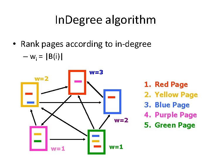
In. Degree algorithm • Rank pages according to in-degree – wi = |B(i)| w=3 w=2 w=1 1. 2. 3. 4. 5. Red Page Yellow Page Blue Page Purple Page Green Page

Page. Rank algorithm [BP 98] • Good authorities should be pointed by good authorities • Random walk on the web graph – pick a page at random – with probability 1 - α jump to a random page – with probability α follow a random outgoing link • Rank according to the stationary distribution • 1. 2. 3. 4. 5. Red Page Purple Page Yellow Page Blue Page Green Page

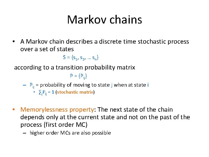
Markov chains • A Markov chain describes a discrete time stochastic process over a set of states S = {s 1, s 2, … sn} according to a transition probability matrix P = {Pij} – Pij = probability of moving to state j when at state i • ∑j. Pij = 1 (stochastic matrix) • Memorylessness property: The next state of the chain depends only at the current state and not on the past of the process (first order MC) – higher order MCs are also possible

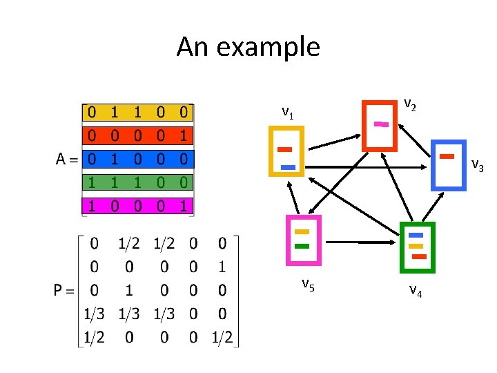
Random walks • Random walks on graphs correspond to Markov Chains – The set of states S is the set of nodes of the graph G – The transition probability matrix is the probability that we follow an edge from one node to another

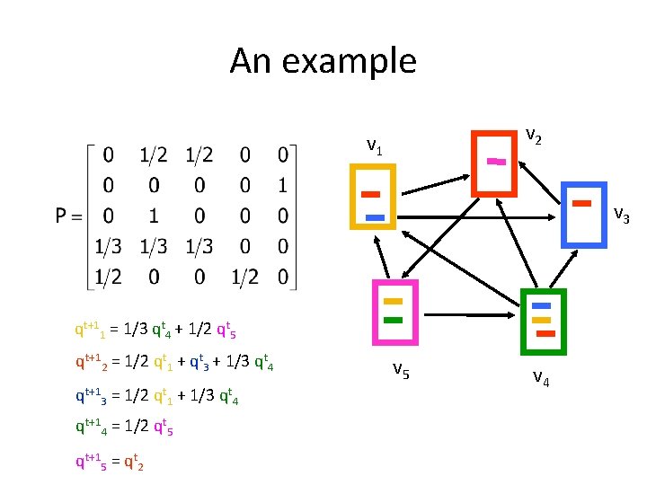
An example v 2 v 1 v 3 v 5 v 4

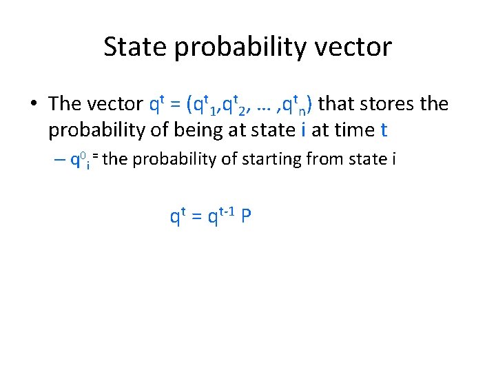
State probability vector • The vector qt = (qt 1, qt 2, … , qtn) that stores the probability of being at state i at time t – q 0 i = the probability of starting from state i qt = qt-1 P

An example v 2 v 1 v 3 qt+11 = 1/3 qt 4 + 1/2 qt 5 qt+12 = 1/2 qt 1 + qt 3 + 1/3 qt 4 qt+13 = 1/2 qt 1 + 1/3 qt 4 qt+14 = 1/2 qt 5 qt+15 = qt 2 v 5 v 4

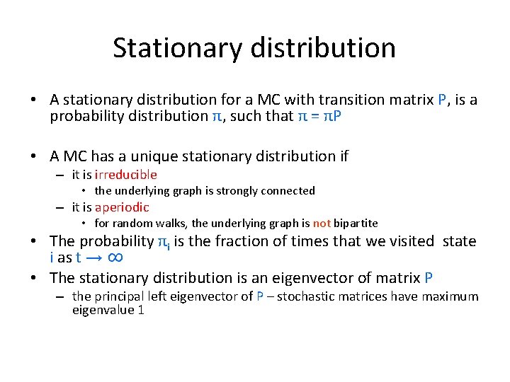
Stationary distribution • A stationary distribution for a MC with transition matrix P, is a probability distribution π, such that π = πP • A MC has a unique stationary distribution if – it is irreducible • the underlying graph is strongly connected – it is aperiodic • for random walks, the underlying graph is not bipartite • The probability πi is the fraction of times that we visited state i as t → ∞ • The stationary distribution is an eigenvector of matrix P – the principal left eigenvector of P – stochastic matrices have maximum eigenvalue 1

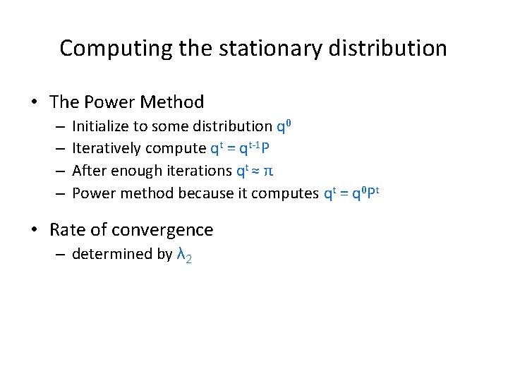
Computing the stationary distribution • The Power Method – – Initialize to some distribution q 0 Iteratively compute qt = qt-1 P After enough iterations qt ≈ π Power method because it computes qt = q 0 Pt • Rate of convergence – determined by λ 2

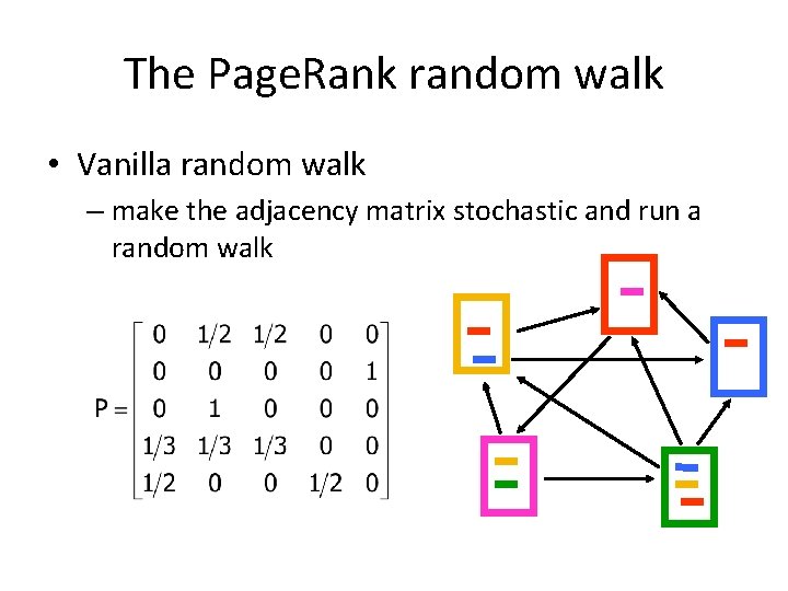
The Page. Rank random walk • Vanilla random walk – make the adjacency matrix stochastic and run a random walk

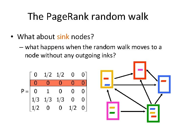
The Page. Rank random walk • What about sink nodes? – what happens when the random walk moves to a node without any outgoing inks?

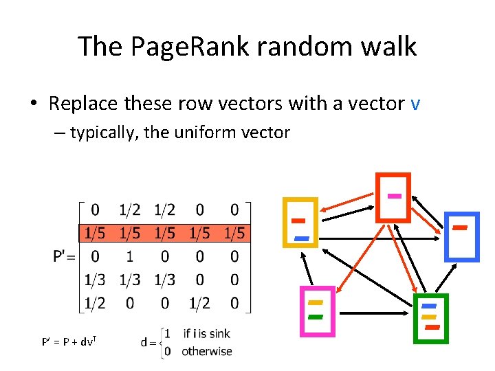
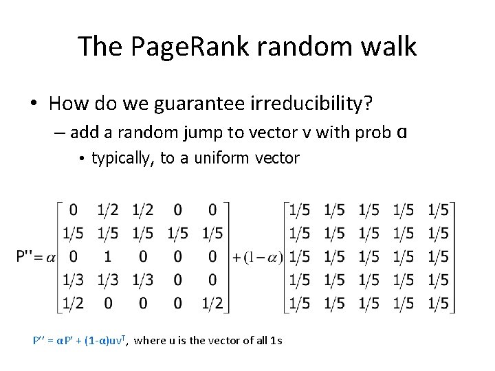
The Page. Rank random walk • Replace these row vectors with a vector v – typically, the uniform vector P’ = P + dv. T

The Page. Rank random walk • How do we guarantee irreducibility? – add a random jump to vector v with prob α • typically, to a uniform vector P’’ = αP’ + (1 -α)uv. T, where u is the vector of all 1 s

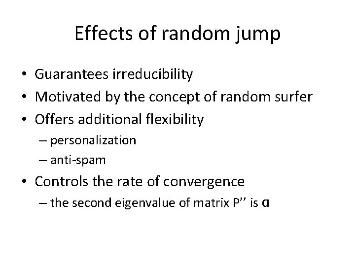
Effects of random jump • Guarantees irreducibility • Motivated by the concept of random surfer • Offers additional flexibility – personalization – anti-spam • Controls the rate of convergence – the second eigenvalue of matrix P’’ is α

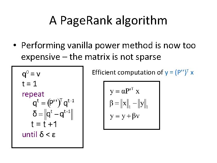
A Page. Rank algorithm • Performing vanilla power method is now too expensive – the matrix is not sparse q 0 = v t=1 repeat t = t +1 until δ < ε Efficient computation of y = (P’’)T x

Random walks on undirected graphs • In the stationary distribution of a random walk on an undirected graph, the probability of being at node i is proportional to the (weighted) degree of the vertex • Random walks on undirected graphs are not “interesting”

Research on Page. Rank • Specialized Page. Rank – personalization [BP 98] • instead of picking a node uniformly at random favor specific nodes that are related to the user – topic sensitive Page. Rank [H 02] • compute many Page. Rank vectors, one for each topic • estimate relevance of query with each topic • produce final Page. Rank as a weighted combination • Updating Page. Rank [Chien et al 2002] • Fast computation of Page. Rank – numerical analysis tricks – node aggregation techniques – dealing with the “Web frontier”

Topic-sensitive pagerank • HITS-based scores are very inefficient to compute • Page. Rank scores are independent of the queries • Can we bias Page. Rank rankings to take into account query keywords? Topic-sensitive Page. Rank

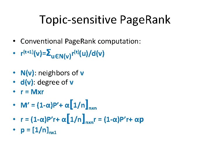
Topic-sensitive Page. Rank • Conventional Page. Rank computation: • r(t+1)(v)=ΣuЄN(v)r(t)(u)/d(v) • N(v): neighbors of v • d(v): degree of v • r = Mxr • M’ = (1 -α)P’+ α[1/n]nxn • r = (1 -α)P’r+ α[1/n]nxnr = (1 -α)P’r+ αp • p = [1/n]nx 1

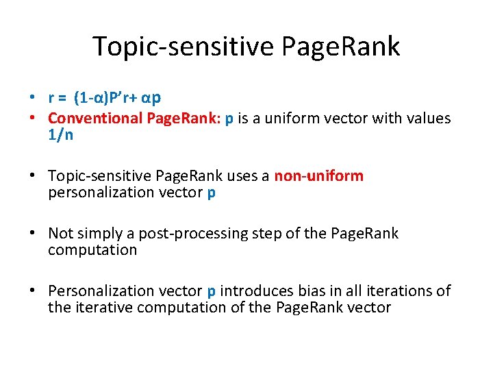
Topic-sensitive Page. Rank • r = (1 -α)P’r+ αp • Conventional Page. Rank: p is a uniform vector with values 1/n • Topic-sensitive Page. Rank uses a non-uniform personalization vector p • Not simply a post-processing step of the Page. Rank computation • Personalization vector p introduces bias in all iterations of the iterative computation of the Page. Rank vector

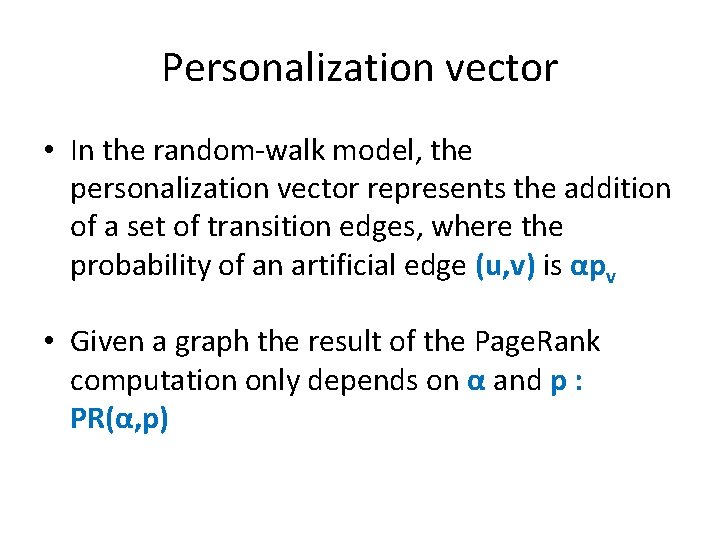
Personalization vector • In the random-walk model, the personalization vector represents the addition of a set of transition edges, where the probability of an artificial edge (u, v) is αpv • Given a graph the result of the Page. Rank computation only depends on α and p : PR(α, p)

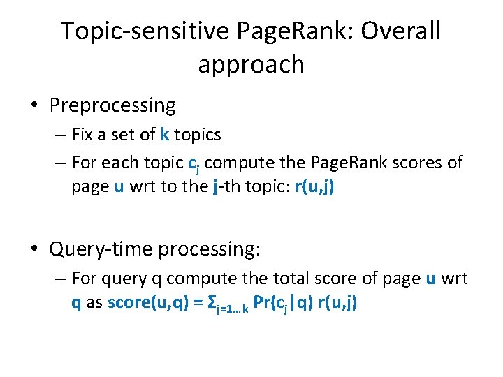
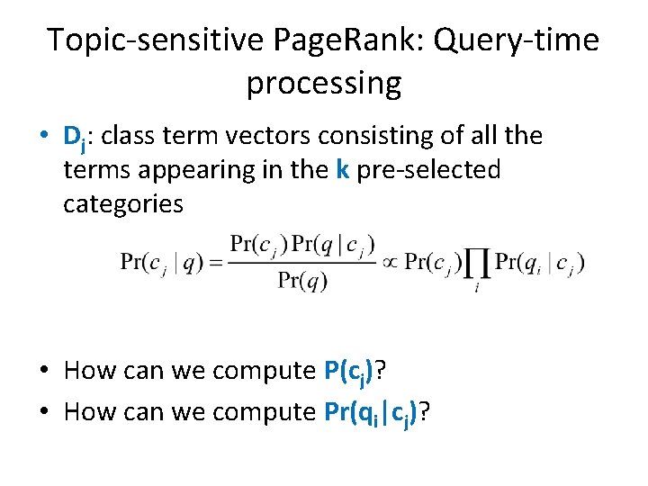
Topic-sensitive Page. Rank: Overall approach • Preprocessing – Fix a set of k topics – For each topic cj compute the Page. Rank scores of page u wrt to the j-th topic: r(u, j) • Query-time processing: – For query q compute the total score of page u wrt q as score(u, q) = Σj=1…k Pr(cj|q) r(u, j)

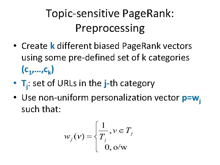
Topic-sensitive Page. Rank: Preprocessing • Create k different biased Page. Rank vectors using some pre-defined set of k categories (c 1, …, ck) • Tj: set of URLs in the j-th category • Use non-uniform personalization vector p=wj such that:

Topic-sensitive Page. Rank: Query-time processing • Dj: class term vectors consisting of all the terms appearing in the k pre-selected categories • How can we compute P(cj)? • How can we compute Pr(qi|cj)?

• Comparing results of Link Analysis Ranking algorithms • Comparing and aggregating rankings

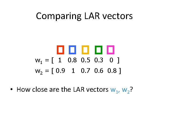
Comparing LAR vectors w 1 = [ 1 0. 8 0. 5 0. 3 0 ] w 2 = [ 0. 9 1 0. 7 0. 6 0. 8 ] • How close are the LAR vectors w 1, w 2?

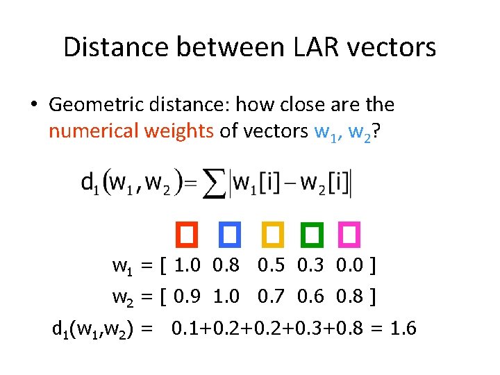
Distance between LAR vectors • Geometric distance: how close are the numerical weights of vectors w 1, w 2? w 1 = [ 1. 0 0. 8 0. 5 0. 3 0. 0 ] w 2 = [ 0. 9 1. 0 0. 7 0. 6 0. 8 ] d 1(w 1, w 2) = 0. 1+0. 2+0. 3+0. 8 = 1. 6

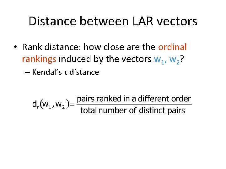
Distance between LAR vectors • Rank distance: how close are the ordinal rankings induced by the vectors w 1, w 2? – Kendal’s τ distance

Outline • Rank Aggregation – Computing aggregate scores – Computing aggregate rankings - voting

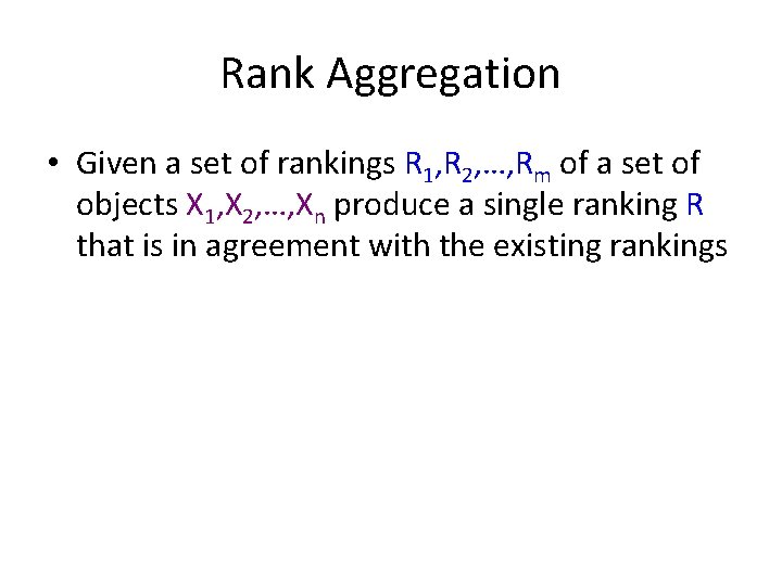
Rank Aggregation • Given a set of rankings R 1, R 2, …, Rm of a set of objects X 1, X 2, …, Xn produce a single ranking R that is in agreement with the existing rankings

Examples • Voting – rankings R 1, R 2, …, Rm are the voters, the objects X 1, X 2, …, Xn are the candidates.

Examples • Combining multiple scoring functions – rankings R 1, R 2, …, Rm are the scoring functions, the objects X 1, X 2, …, Xn are data items. • Combine the Page. Rank scores with term-weighting scores • Combine scores for multimedia items – color, shape, texture • Combine scores for database tuples – find the best hotel according to price and location

Examples • Combining multiple sources – rankings R 1, R 2, …, Rm are the sources, the objects X 1, X 2, …, Xn are data items. • meta-search engines for the Web • distributed databases • P 2 P sources

Variants of the problem • Combining scores – we know the scores assigned to objects by each ranking, and we want to compute a single score • Combining ordinal rankings – the scores are not known, only the ordering is known – the scores are known but we do not know how, or do not want to combine them • e. g. price and star rating

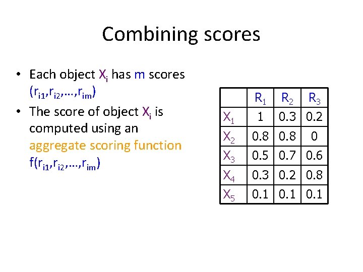
Combining scores • Each object Xi has m scores (ri 1, ri 2, …, rim) • The score of object Xi is computed using an aggregate scoring function f(ri 1, ri 2, …, rim) X 1 R 2 R 3 1 0. 3 0. 2 X 2 0. 8 0 X 3 0. 5 0. 7 0. 6 X 4 0. 3 0. 2 0. 8 X 5 0. 1

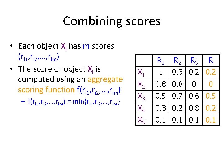
Combining scores • Each object Xi has m scores (ri 1, ri 2, …, rim) • The score of object Xi is computed using an aggregate scoring function f(ri 1, ri 2, …, rim) – f(ri 1, ri 2, …, rim) = min{ri 1, ri 2, …, rim} X 1 R 2 R 3 1 0. 3 0. 2 0 R X 2 0. 8 0 X 3 0. 5 0. 7 0. 6 0. 5 X 4 0. 3 0. 2 0. 8 0. 2 X 5 0. 1

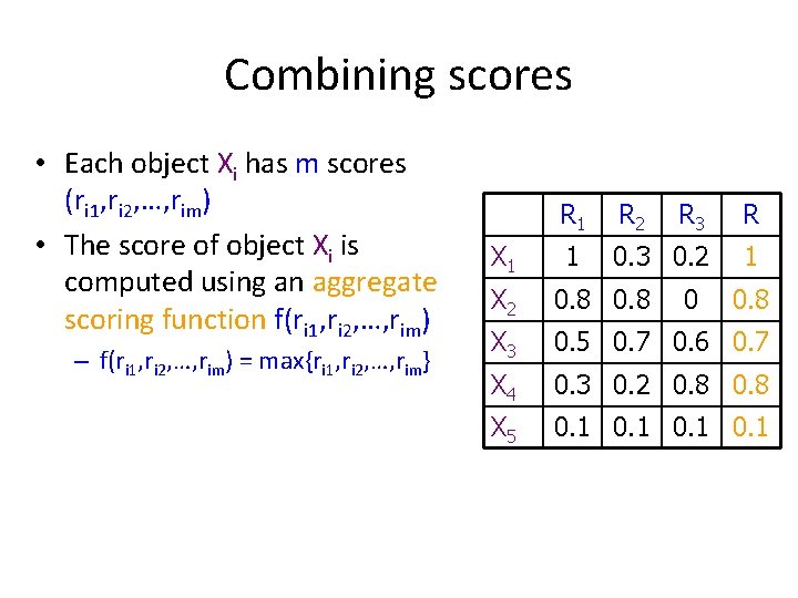
Combining scores • Each object Xi has m scores (ri 1, ri 2, …, rim) • The score of object Xi is computed using an aggregate scoring function f(ri 1, ri 2, …, rim) – f(ri 1, ri 2, …, rim) = max{ri 1, ri 2, …, rim} X 1 R 2 R 3 R 1 0. 3 0. 2 1 X 2 0. 8 0 0. 8 X 3 0. 5 0. 7 0. 6 0. 7 X 4 0. 3 0. 2 0. 8 X 5 0. 1

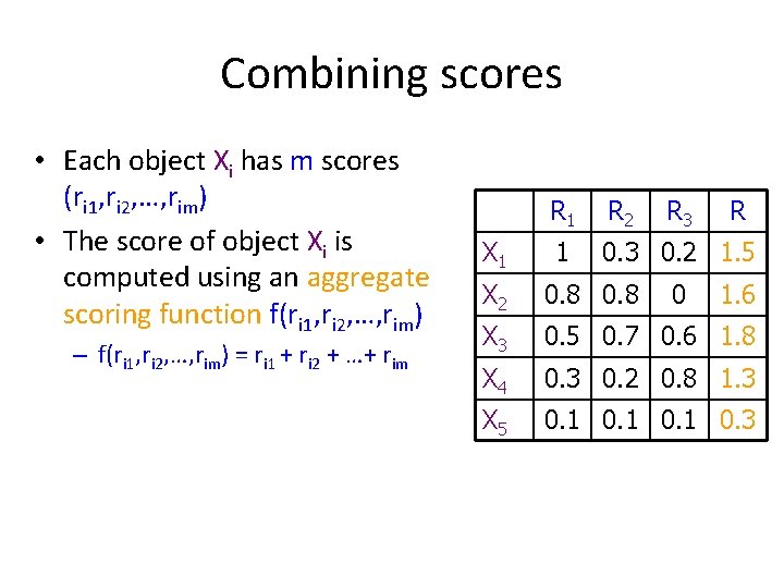
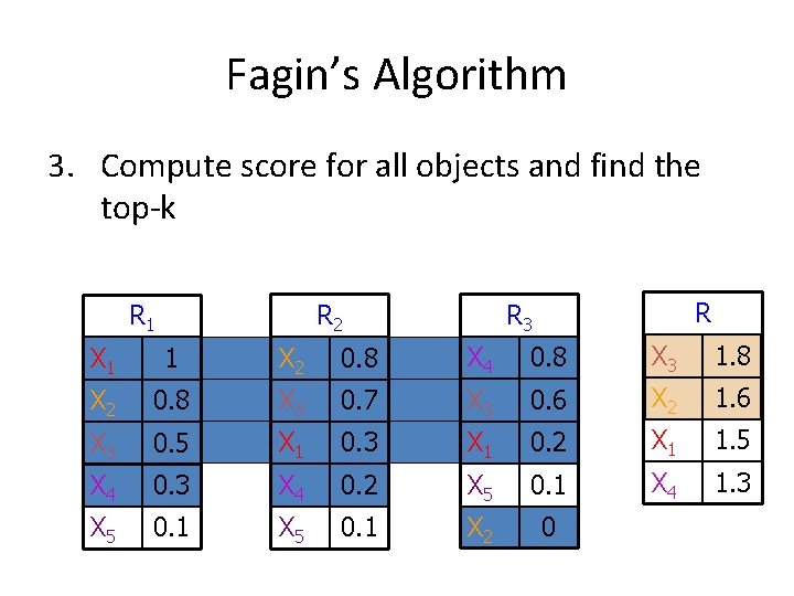
Combining scores • Each object Xi has m scores (ri 1, ri 2, …, rim) • The score of object Xi is computed using an aggregate scoring function f(ri 1, ri 2, …, rim) – f(ri 1, ri 2, …, rim) = ri 1 + ri 2 + …+ rim X 1 R 2 R 3 1 0. 3 0. 2 1. 5 0 R X 2 0. 8 1. 6 X 3 0. 5 0. 7 0. 6 1. 8 X 4 0. 3 0. 2 0. 8 1. 3 X 5 0. 1 0. 3

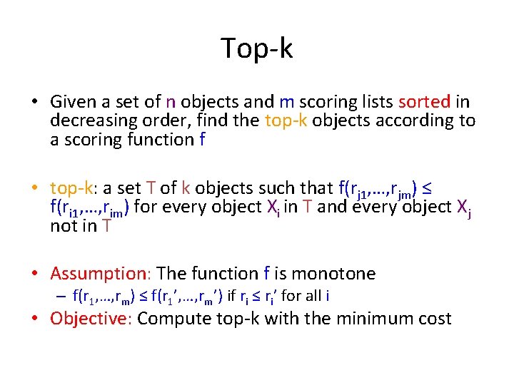
Top-k • Given a set of n objects and m scoring lists sorted in decreasing order, find the top-k objects according to a scoring function f • top-k: a set T of k objects such that f(rj 1, …, rjm) ≤ f(ri 1, …, rim) for every object Xi in T and every object Xj not in T • Assumption: The function f is monotone – f(r 1, …, rm) ≤ f(r 1’, …, rm’) if ri ≤ ri’ for all i • Objective: Compute top-k with the minimum cost

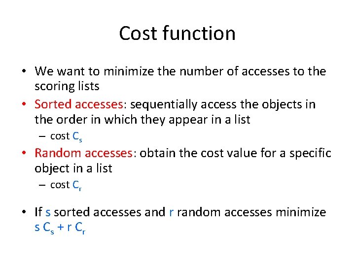
Cost function • We want to minimize the number of accesses to the scoring lists • Sorted accesses: sequentially access the objects in the order in which they appear in a list – cost Cs • Random accesses: obtain the cost value for a specific object in a list – cost Cr • If s sorted accesses and r random accesses minimize s Cs + r C r

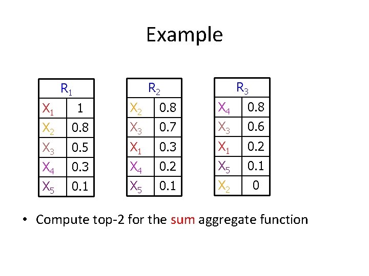
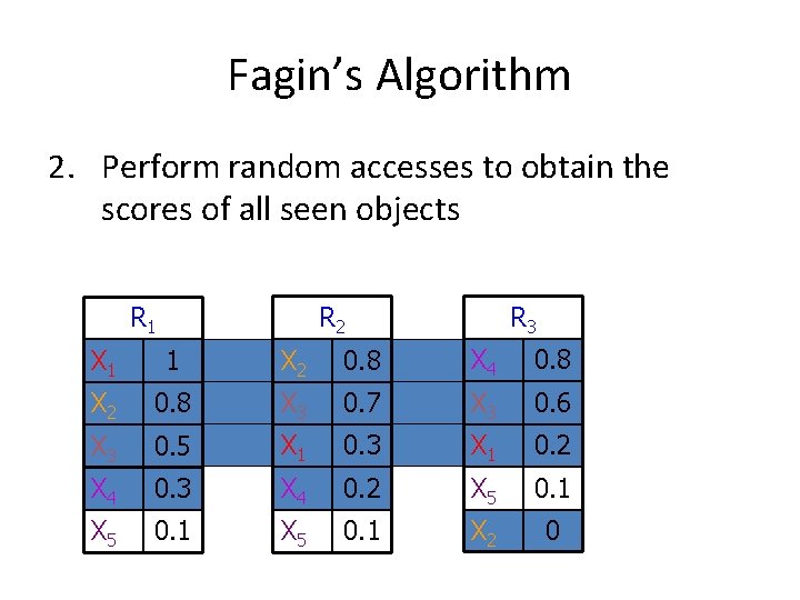
Example R 3 R 2 R 1 X 1 1 X 2 0. 8 X 4 0. 8 X 2 0. 8 X 3 0. 7 X 3 0. 6 X 3 0. 5 X 1 0. 3 X 1 0. 2 X 4 0. 3 X 4 0. 2 X 5 0. 1 X 2 0 • Compute top-2 for the sum aggregate function

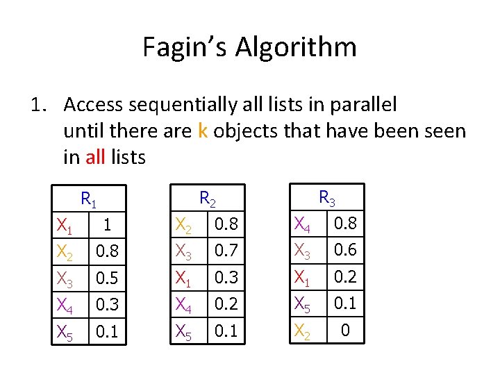
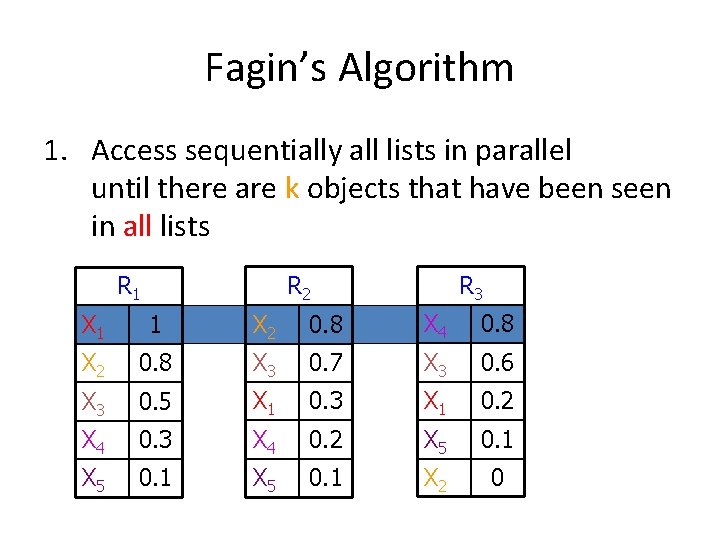
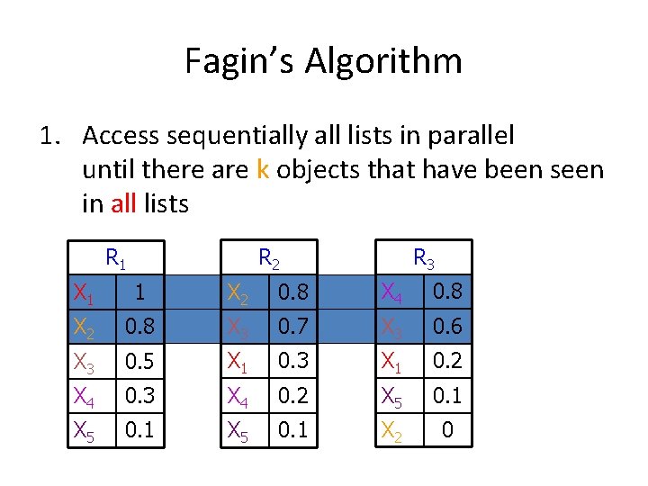
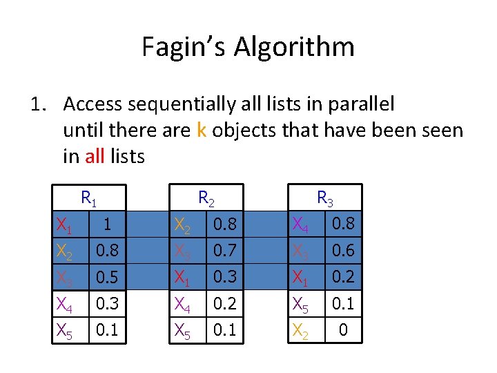
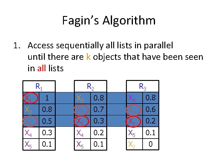
Fagin’s Algorithm 1. Access sequentially all lists in parallel until there are k objects that have been seen in all lists R 3 R 2 R 1 X 1 1 X 2 0. 8 X 4 0. 8 X 2 0. 8 X 3 0. 7 X 3 0. 6 X 3 0. 5 X 1 0. 3 X 1 0. 2 X 4 0. 3 X 4 0. 2 X 5 0. 1 X 2 0

Fagin’s Algorithm 1. Access sequentially all lists in parallel until there are k objects that have been seen in all lists R 3 R 2 R 1 X 1 1 X 2 0. 8 X 4 0. 8 X 2 0. 8 X 3 0. 7 X 3 0. 6 X 3 0. 5 X 1 0. 3 X 1 0. 2 X 4 0. 3 X 4 0. 2 X 5 0. 1 X 2 0

Fagin’s Algorithm 1. Access sequentially all lists in parallel until there are k objects that have been seen in all lists R 3 R 2 R 1 X 1 1 X 2 0. 8 X 4 0. 8 X 2 0. 8 X 3 0. 7 X 3 0. 6 X 3 0. 5 X 1 0. 3 X 1 0. 2 X 4 0. 3 X 4 0. 2 X 5 0. 1 X 2 0

Fagin’s Algorithm 1. Access sequentially all lists in parallel until there are k objects that have been seen in all lists R 3 R 2 R 1 X 1 1 X 2 0. 8 X 4 0. 8 X 2 0. 8 X 3 0. 7 X 3 0. 6 X 3 0. 5 X 1 0. 3 X 1 0. 2 X 4 0. 3 X 4 0. 2 X 5 0. 1 X 2 0

Fagin’s Algorithm 1. Access sequentially all lists in parallel until there are k objects that have been seen in all lists R 3 R 2 R 1 X 1 1 X 2 0. 8 X 4 0. 8 X 2 0. 8 X 3 0. 7 X 3 0. 6 X 3 0. 5 X 1 0. 3 X 1 0. 2 X 4 0. 3 X 4 0. 2 X 5 0. 1 X 2 0

Fagin’s Algorithm 2. Perform random accesses to obtain the scores of all seen objects R 3 R 2 R 1 X 1 1 X 2 0. 8 X 4 0. 8 X 2 0. 8 X 3 0. 7 X 3 0. 6 X 3 0. 5 X 1 0. 3 X 1 0. 2 X 4 0. 3 X 4 0. 2 X 5 0. 1 X 2 0

Fagin’s Algorithm 3. Compute score for all objects and find the top-k R R 3 R 2 R 1 X 1 1 X 2 0. 8 X 4 0. 8 X 3 1. 8 X 2 0. 8 X 3 0. 7 X 3 0. 6 X 2 1. 6 X 3 0. 5 X 1 0. 3 X 1 0. 2 X 1 1. 5 X 4 0. 3 X 4 0. 2 X 5 0. 1 X 4 1. 3 X 5 0. 1 X 2 0

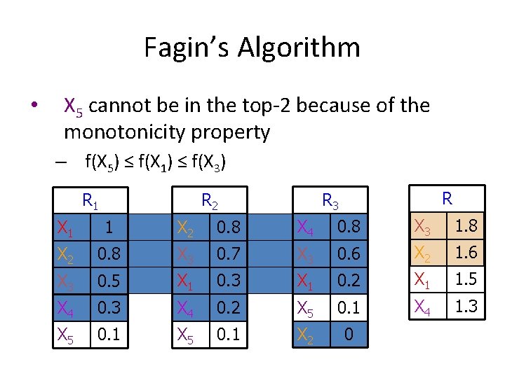
Fagin’s Algorithm • X 5 cannot be in the top-2 because of the monotonicity property – f(X 5) ≤ f(X 1) ≤ f(X 3) R R 3 R 2 R 1 X 1 1 X 2 0. 8 X 4 0. 8 X 3 1. 8 X 2 0. 8 X 3 0. 7 X 3 0. 6 X 2 1. 6 X 3 0. 5 X 1 0. 3 X 1 0. 2 X 1 1. 5 X 4 0. 3 X 4 0. 2 X 5 0. 1 X 4 1. 3 X 5 0. 1 X 2 0

Fagin’s Algorithm • The algorithm is cost optimal under some probabilistic assumptions for a restricted class of aggregate functions

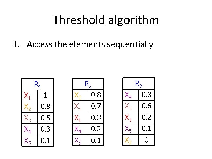
Threshold algorithm 1. Access the elements sequentially R 3 R 2 R 1 X 1 1 X 2 0. 8 X 4 0. 8 X 2 0. 8 X 3 0. 7 X 3 0. 6 X 3 0. 5 X 1 0. 3 X 1 0. 2 X 4 0. 3 X 4 0. 2 X 5 0. 1 X 2 0

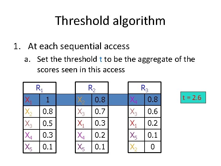
Threshold algorithm 1. At each sequential access a. Set the threshold t to be the aggregate of the scores seen in this access R 3 R 2 R 1 X 1 1 X 2 0. 8 X 4 0. 8 X 2 0. 8 X 3 0. 7 X 3 0. 6 X 3 0. 5 X 1 0. 3 X 1 0. 2 X 4 0. 3 X 4 0. 2 X 5 0. 1 X 2 0 t = 2. 6

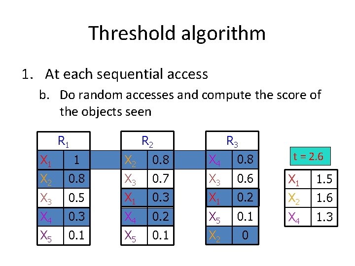
Threshold algorithm 1. At each sequential access b. Do random accesses and compute the score of the objects seen R 3 R 2 R 1 t = 2. 6 X 1 1 X 2 0. 8 X 4 0. 8 X 2 0. 8 X 3 0. 7 X 3 0. 6 X 1 1. 5 X 3 0. 5 X 1 0. 3 X 1 0. 2 X 2 1. 6 X 4 0. 3 X 4 0. 2 X 5 0. 1 X 4 1. 3 X 5 0. 1 X 2 0

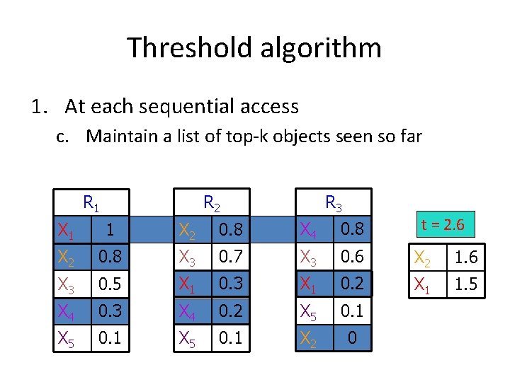
Threshold algorithm 1. At each sequential access c. Maintain a list of top-k objects seen so far R 3 R 2 R 1 t = 2. 6 X 1 1 X 2 0. 8 X 4 0. 8 X 2 0. 8 X 3 0. 7 X 3 0. 6 X 2 1. 6 X 3 0. 5 X 1 0. 3 X 1 0. 2 X 1 1. 5 X 4 0. 3 X 4 0. 2 X 5 0. 1 X 2 0

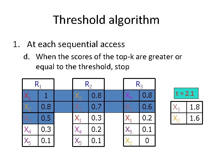
Threshold algorithm 1. At each sequential access d. When the scores of the top-k are greater or equal to the threshold, stop R 3 R 2 R 1 t = 2. 1 X 1 1 X 2 0. 8 X 4 0. 8 X 2 0. 8 X 3 0. 7 X 3 0. 6 X 3 1. 8 X 3 0. 5 X 1 0. 3 X 1 0. 2 X 2 1. 6 X 4 0. 3 X 4 0. 2 X 5 0. 1 X 2 0

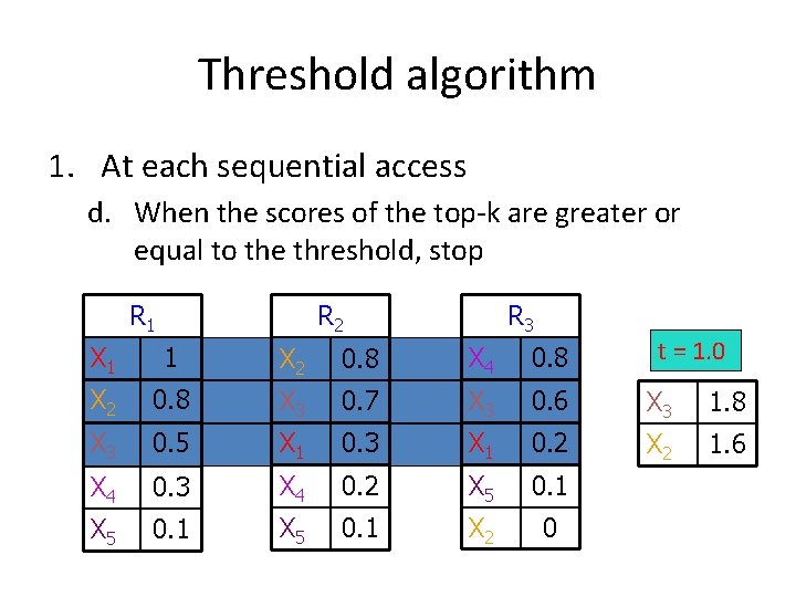
Threshold algorithm 1. At each sequential access d. When the scores of the top-k are greater or equal to the threshold, stop R 1 R 3 R 2 t = 1. 0 X 1 1 X 2 0. 8 X 4 0. 8 X 2 0. 8 X 3 0. 7 X 3 0. 6 X 3 1. 8 X 3 0. 5 X 1 0. 3 X 1 0. 2 X 2 1. 6 X 4 0. 3 X 4 0. 2 X 5 0. 1 X 2 0

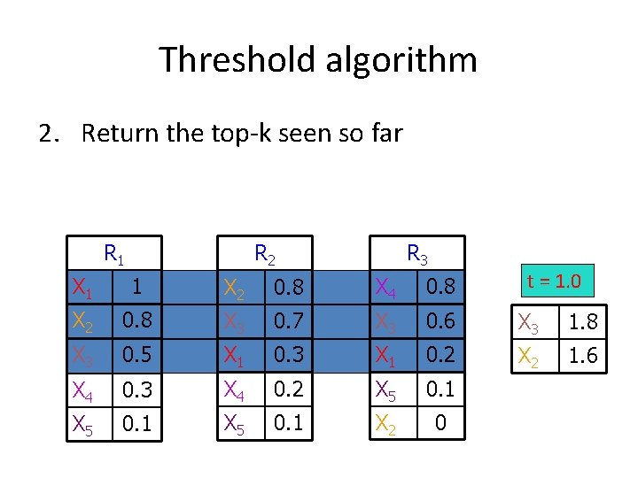
Threshold algorithm 2. Return the top-k seen so far R 1 R 3 R 2 t = 1. 0 X 1 1 X 2 0. 8 X 4 0. 8 X 2 0. 8 X 3 0. 7 X 3 0. 6 X 3 1. 8 X 3 0. 5 X 1 0. 3 X 1 0. 2 X 2 1. 6 X 4 0. 3 X 4 0. 2 X 5 0. 1 X 2 0

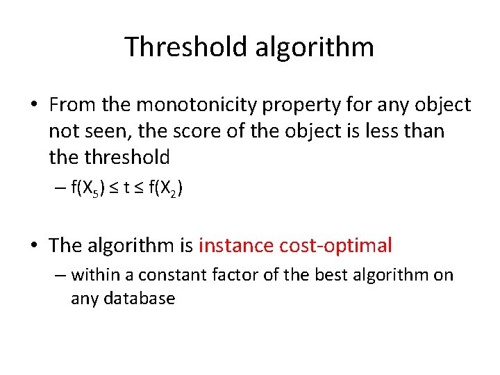
Threshold algorithm • From the monotonicity property for any object not seen, the score of the object is less than the threshold – f(X 5) ≤ t ≤ f(X 2) • The algorithm is instance cost-optimal – within a constant factor of the best algorithm on any database

Combining rankings • In many cases the scores are not known – e. g. meta-search engines – scores are proprietary information • … or we do not know how they were obtained – one search engine returns score 10, the other 100. What does this mean? • … or the scores are incompatible – apples and oranges: does it make sense to combine price with distance? • In this cases we can only work with the rankings

The problem • Input: a set of rankings R 1, R 2, …, Rm of the objects X 1, X 2, …, Xn. Each ranking Ri is a total ordering of the objects – for every pair Xi, Xj either Xi is ranked above Xj or Xj is ranked above Xi • Output: A total ordering R that aggregates rankings R 1, R 2, …, Rm

Voting theory • A voting system is a rank aggregation mechanism • Long history and literature – criteria and axioms for good voting systems

What is a good voting system? • The Condorcet criterion – if object A defeats every other object in a pairwise majority vote, then A should be ranked first • Extended Condorcet criterion – if the objects in a set X defeat in pairwise comparisons the objects in the set Y then the objects in X should be ranked above those in Y • Not all voting systems satisfy the Condorcet criterion!

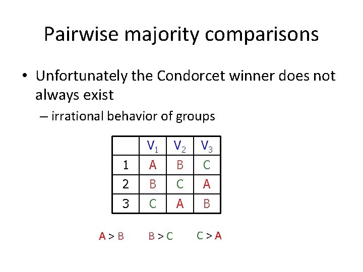
Pairwise majority comparisons • Unfortunately the Condorcet winner does not always exist – irrational behavior of groups V 1 V 2 V 3 1 A B C 2 B C A 3 C A B A>B B>C C>A

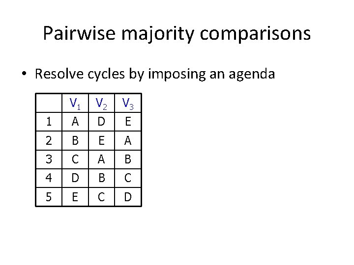
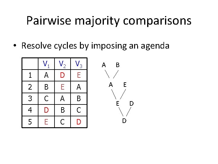
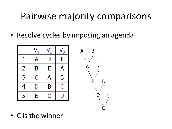
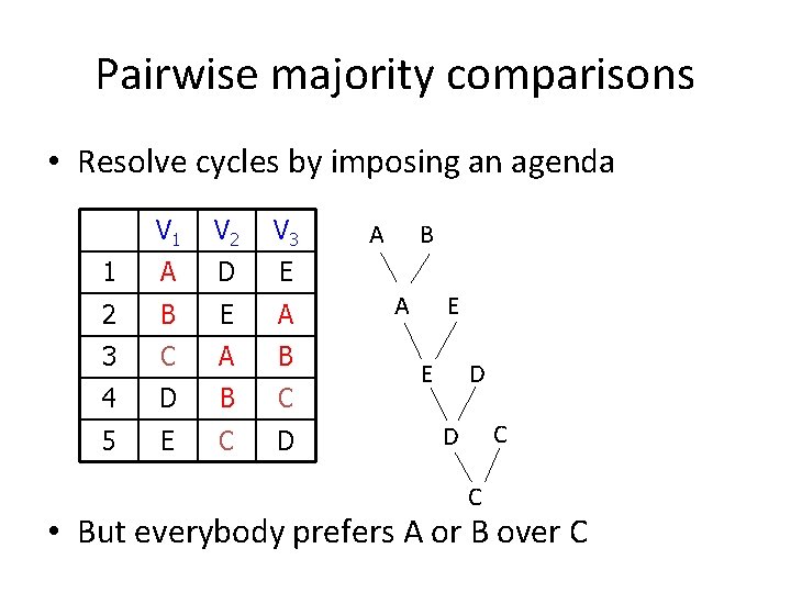
Pairwise majority comparisons • Resolve cycles by imposing an agenda V 1 V 2 V 3 1 A D E 2 B E A 3 C A B 4 D B C 5 E C D

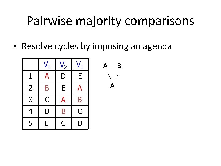
Pairwise majority comparisons • Resolve cycles by imposing an agenda V 1 V 2 V 3 1 A D E 2 B E A 3 C A B 4 D B C 5 E C D B A A

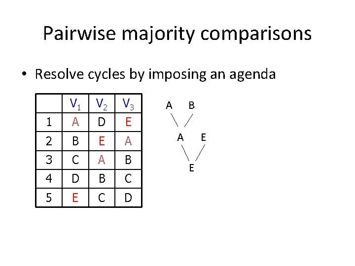
Pairwise majority comparisons • Resolve cycles by imposing an agenda V 1 V 2 V 3 1 A D E 2 B E A 3 C A B 4 D B C 5 E C D B A E

Pairwise majority comparisons • Resolve cycles by imposing an agenda V 1 V 2 V 3 1 A D E 2 B E A 3 C A B 4 D B C 5 E C D B A E A D E D

Pairwise majority comparisons • Resolve cycles by imposing an agenda V 1 V 2 V 3 1 A D E 2 B E A 3 C A B 4 D B C 5 E C D • C is the winner B A E A D E C D C

Pairwise majority comparisons • Resolve cycles by imposing an agenda V 1 V 2 V 3 1 A D E 2 B E A 3 C A B 4 D B C 5 E C D B A E A D E C D C • But everybody prefers A or B over C

Pairwise majority comparisons • The voting system is not Pareto optimal – there exists another ordering that everybody prefers • Also, it is sensitive to the order of voting

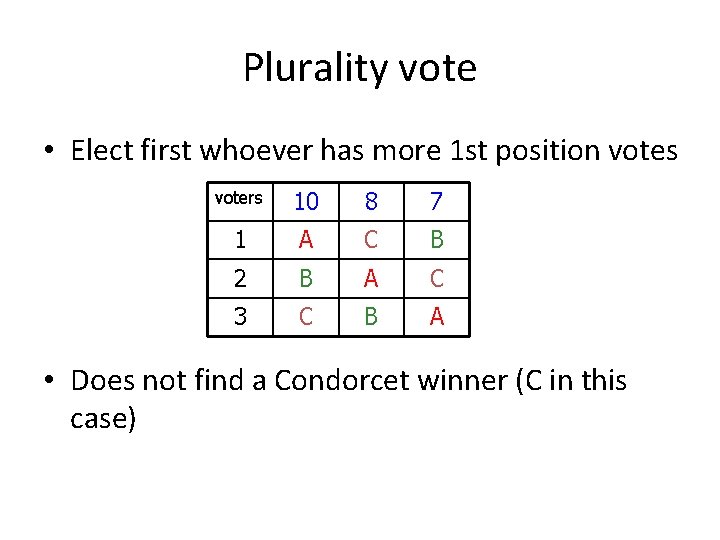
Plurality vote • Elect first whoever has more 1 st position votes voters 10 8 7 1 A C B 2 B A C 3 C B A • Does not find a Condorcet winner (C in this case)

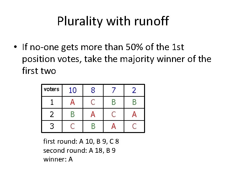
Plurality with runoff • If no-one gets more than 50% of the 1 st position votes, take the majority winner of the first two voters 10 8 7 2 1 A C B B 2 B A C A 3 C B A C first round: A 10, B 9, C 8 second round: A 18, B 9 winner: A

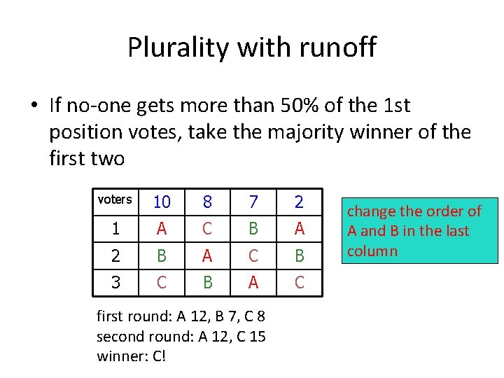
Plurality with runoff • If no-one gets more than 50% of the 1 st position votes, take the majority winner of the first two voters 10 8 7 2 1 A C B A 2 B A C B 3 C B A C first round: A 12, B 7, C 8 second round: A 12, C 15 winner: C! change the order of A and B in the last column

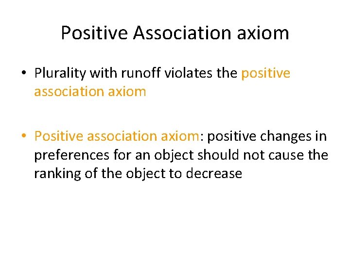
Positive Association axiom • Plurality with runoff violates the positive association axiom • Positive association axiom: positive changes in preferences for an object should not cause the ranking of the object to decrease

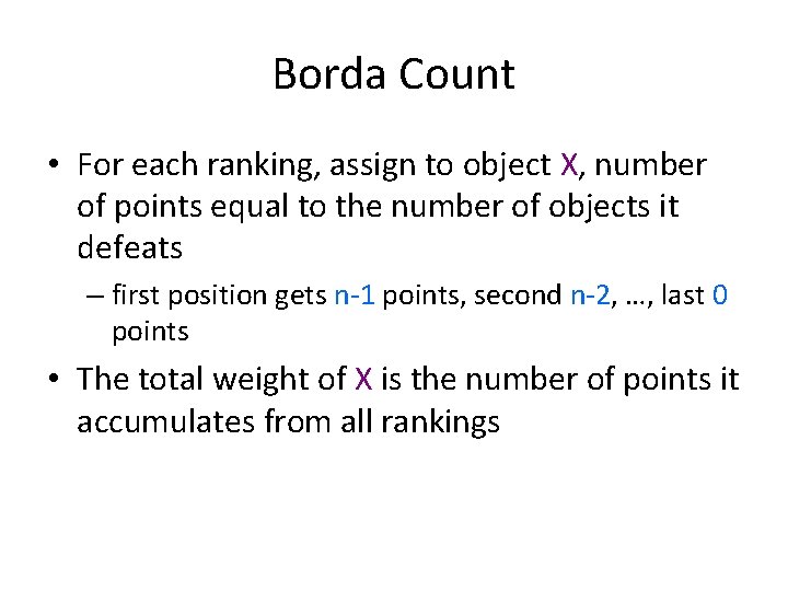
Borda Count • For each ranking, assign to object X, number of points equal to the number of objects it defeats – first position gets n-1 points, second n-2, …, last 0 points • The total weight of X is the number of points it accumulates from all rankings

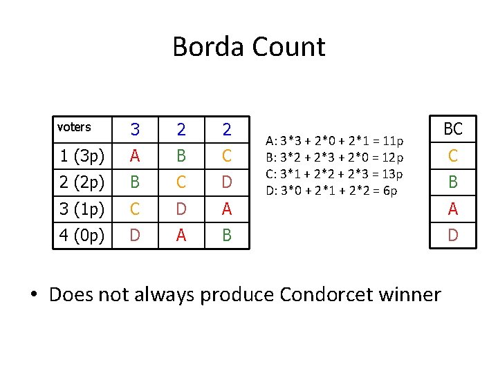
Borda Count voters 3 2 2 1 (3 p) A B C 2 (2 p) B C D 3 (1 p) C D A 4 (0 p) D A B A: 3*3 + 2*0 + 2*1 = 11 p B: 3*2 + 2*3 + 2*0 = 12 p C: 3*1 + 2*2 + 2*3 = 13 p D: 3*0 + 2*1 + 2*2 = 6 p • Does not always produce Condorcet winner BC C B A D

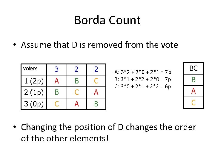
Borda Count • Assume that D is removed from the voters 3 2 2 1 (2 p) A B C 2 (1 p) B C A 3 (0 p) C A B A: 3*2 + 2*0 + 2*1 = 7 p B: 3*1 + 2*2 + 2*0 = 7 p C: 3*0 + 2*1 + 2*2 = 6 p BC B A C • Changing the position of D changes the order of the other elements!

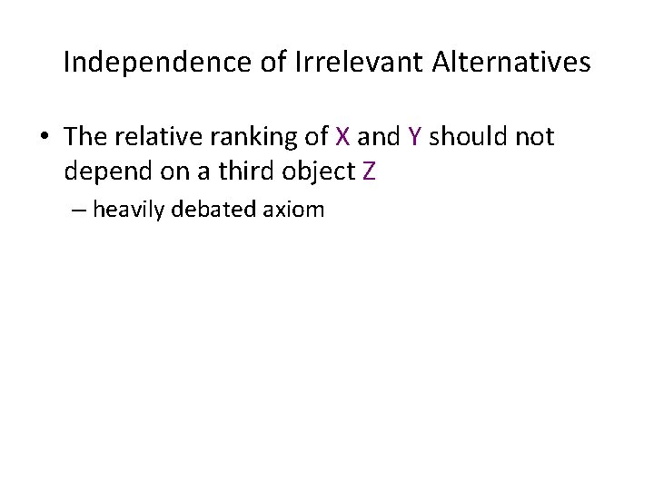
Independence of Irrelevant Alternatives • The relative ranking of X and Y should not depend on a third object Z – heavily debated axiom

Borda Count • The Borda Count of an an object X is the aggregate number of pairwise comparisons that the object X wins – follows from the fact that in one ranking X wins all the pairwise comparisons with objects that are under X in the ranking

Voting Theory • Is there a voting system that does not suffer from the previous shortcomings?

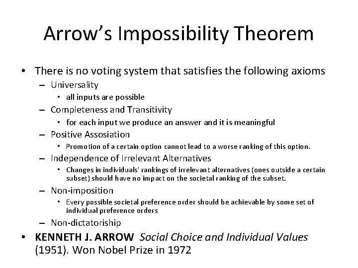
Arrow’s Impossibility Theorem • There is no voting system that satisfies the following axioms – Universality • all inputs are possible – Completeness and Transitivity • for each input we produce an answer and it is meaningful – Positive Assosiation • Promotion of a certain option cannot lead to a worse ranking of this option. – Independence of Irrelevant Alternatives • Changes in individuals' rankings of irrelevant alternatives (ones outside a certain subset) should have no impact on the societal ranking of the subset. – Non-imposition • Every possible societal preference order should be achievable by some set of individual preference orders – Non-dictatoriship • KENNETH J. ARROW Social Choice and Individual Values (1951). Won Nobel Prize in 1972

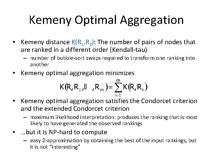
Kemeny Optimal Aggregation • Kemeny distance K(R 1, R 2): The number of pairs of nodes that are ranked in a different order (Kendall-tau) – number of bubble-sort swaps required to transform one ranking into another • Kemeny optimal aggregation minimizes • Kemeny optimal aggregation satisfies the Condorcet criterion and the extended Condorcet criterion – maximum likelihood interpretation: produces the ranking that is most likely to have generated the observed rankings • …but it is NP-hard to compute – easy 2 -approximation by obtaining the best of the input rankings, but it is not “interesting”

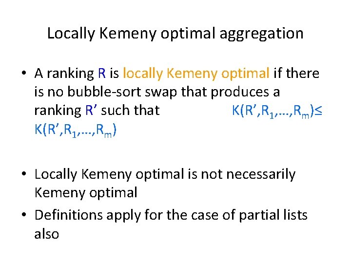
Locally Kemeny optimal aggregation • A ranking R is locally Kemeny optimal if there is no bubble-sort swap that produces a ranking R’ such that K(R’, R 1, …, Rm)≤ K(R’, R 1, …, Rm) • Locally Kemeny optimal is not necessarily Kemeny optimal • Definitions apply for the case of partial lists also

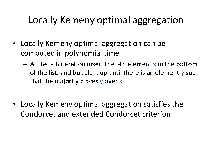
Locally Kemeny optimal aggregation • Locally Kemeny optimal aggregation can be computed in polynomial time – At the i-th iteration insert the i-th element x in the bottom of the list, and bubble it up until there is an element y such that the majority places y over x • Locally Kemeny optimal aggregation satisfies the Condorcet and extended Condorcet criterion

Rank Aggregation algorithm [DKNS 01] • Start with an aggregated ranking and make it into a locally Kemeny optimal aggregation • How do we select the initial aggregation? – Use another aggregation method – Create a Markov Chain where you move from an object X, to another object Y that is ranked higher by the majority

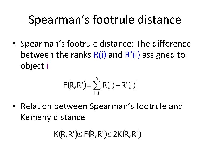
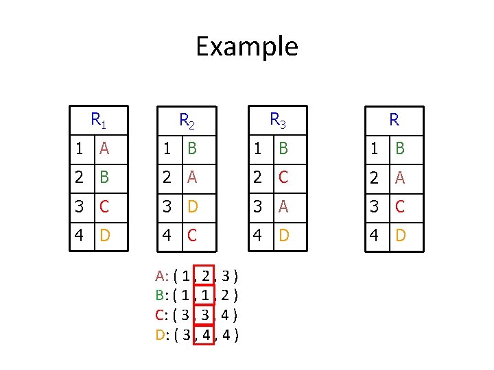
Spearman’s footrule distance • Spearman’s footrule distance: The difference between the ranks R(i) and R’(i) assigned to object i • Relation between Spearman’s footrule and Kemeny distance

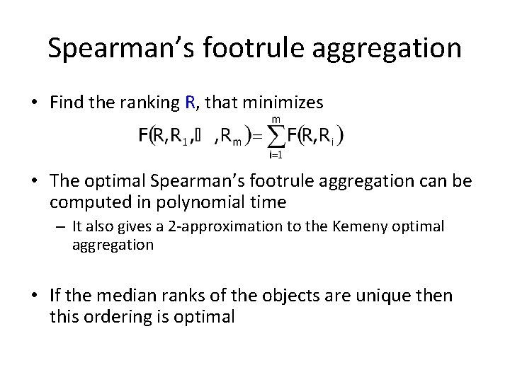
Spearman’s footrule aggregation • Find the ranking R, that minimizes • The optimal Spearman’s footrule aggregation can be computed in polynomial time – It also gives a 2 -approximation to the Kemeny optimal aggregation • If the median ranks of the objects are unique then this ordering is optimal

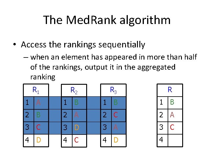
Example R 1 R 2 R 3 1 A 1 B 1 B 2 A 2 C 2 A 3 C 3 D 3 A 3 C 4 D 4 D A: ( 1 , 2 , 3 ) B: ( 1 , 2 ) C: ( 3 , 4 ) D: ( 3 , 4 ) R

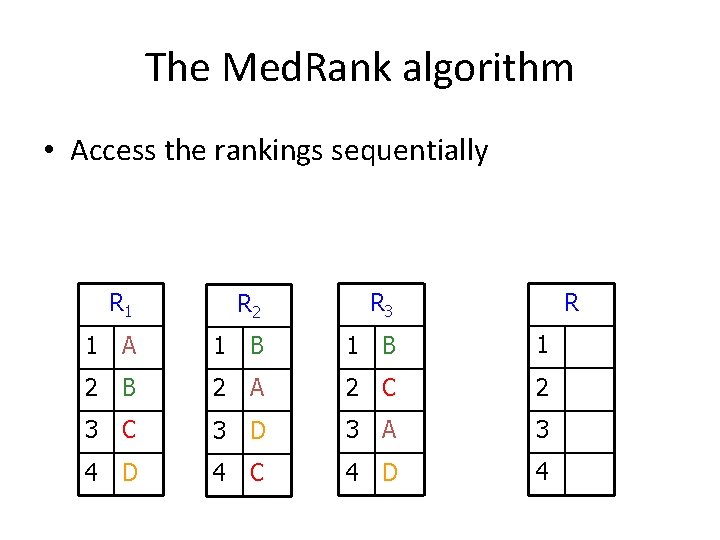
The Med. Rank algorithm • Access the rankings sequentially R R 1 R 2 R 3 1 A 1 B 1 2 B 2 A 2 C 2 3 C 3 D 3 A 3 4 D 4 C 4 D 4

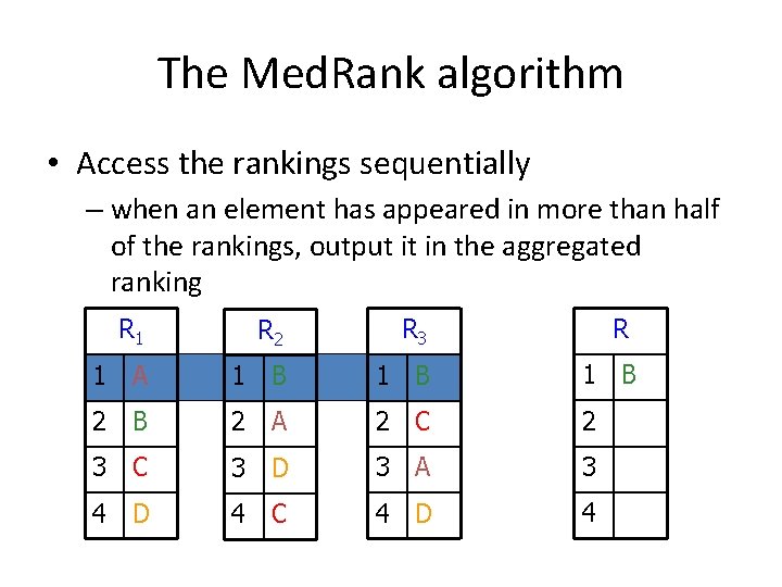
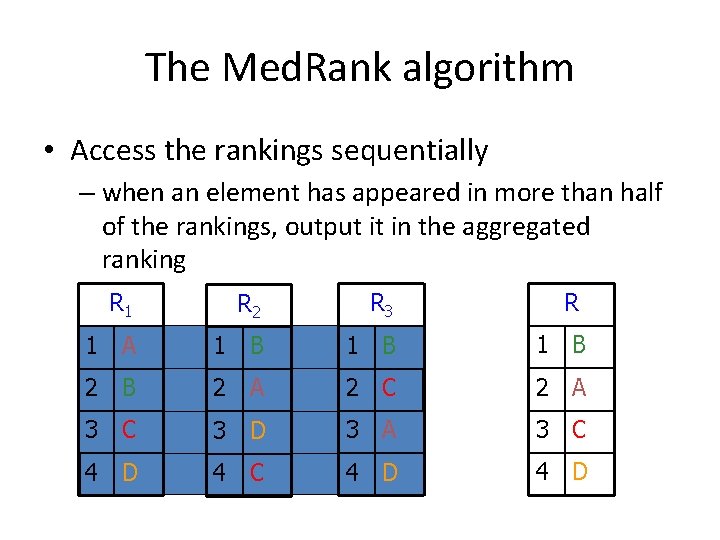
The Med. Rank algorithm • Access the rankings sequentially – when an element has appeared in more than half of the rankings, output it in the aggregated ranking R R 1 R 2 R 3 1 A 1 B 1 B 2 A 2 C 2 3 C 3 D 3 A 3 4 D 4 C 4 D 4

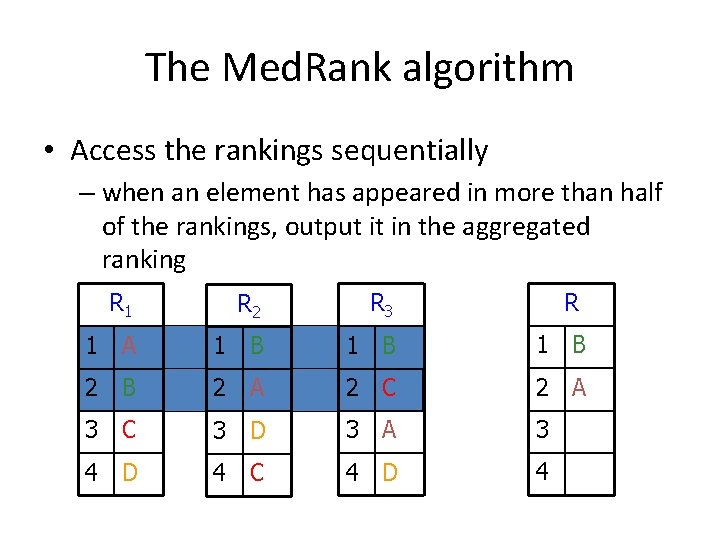
The Med. Rank algorithm • Access the rankings sequentially – when an element has appeared in more than half of the rankings, output it in the aggregated ranking R R 1 R 2 R 3 1 A 1 B 1 B 2 A 2 C 2 A 3 C 3 D 3 A 3 4 D 4 C 4 D 4

The Med. Rank algorithm • Access the rankings sequentially – when an element has appeared in more than half of the rankings, output it in the aggregated ranking R R 1 R 2 R 3 1 A 1 B 1 B 2 A 2 C 2 A 3 C 3 D 3 A 3 C 4 D 4

The Med. Rank algorithm • Access the rankings sequentially – when an element has appeared in more than half of the rankings, output it in the aggregated ranking R R 1 R 2 R 3 1 A 1 B 1 B 2 A 2 C 2 A 3 C 3 D 3 A 3 C 4 D 4 D

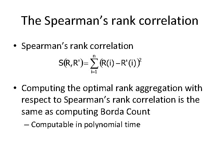
The Spearman’s rank correlation • Spearman’s rank correlation • Computing the optimal rank aggregation with respect to Spearman’s rank correlation is the same as computing Borda Count – Computable in polynomial time

Extensions and Applications • Rank distance measures between partial orderings and top-k lists • Similarity search • Ranked Join Indices • Analysis of Link Analysis Ranking algorithms • Connections with machine learning

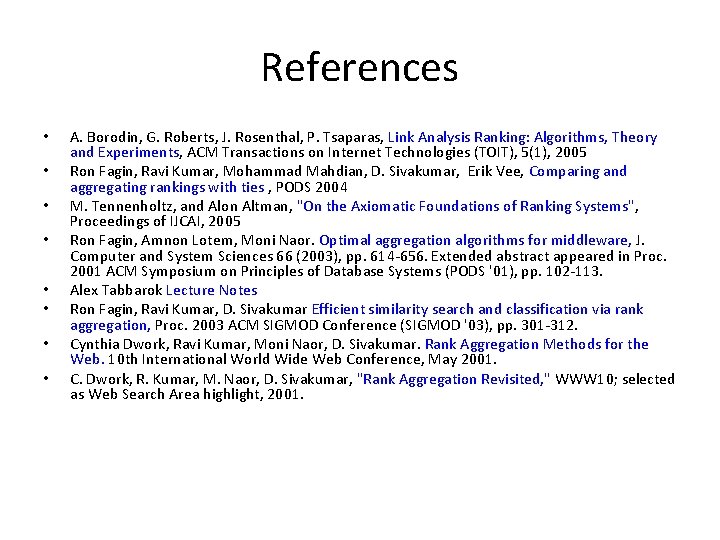
References • • A. Borodin, G. Roberts, J. Rosenthal, P. Tsaparas, Link Analysis Ranking: Algorithms, Theory and Experiments, ACM Transactions on Internet Technologies (TOIT), 5(1), 2005 Ron Fagin, Ravi Kumar, Mohammad Mahdian, D. Sivakumar, Erik Vee, Comparing and aggregating rankings with ties , PODS 2004 M. Tennenholtz, and Alon Altman, "On the Axiomatic Foundations of Ranking Systems", Proceedings of IJCAI, 2005 Ron Fagin, Amnon Lotem, Moni Naor. Optimal aggregation algorithms for middleware, J. Computer and System Sciences 66 (2003), pp. 614 -656. Extended abstract appeared in Proc. 2001 ACM Symposium on Principles of Database Systems (PODS '01), pp. 102 -113. Alex Tabbarok Lecture Notes Ron Fagin, Ravi Kumar, D. Sivakumar Efficient similarity search and classification via rank aggregation, Proc. 2003 ACM SIGMOD Conference (SIGMOD '03), pp. 301 -312. Cynthia Dwork, Ravi Kumar, Moni Naor, D. Sivakumar. Rank Aggregation Methods for the Web. 10 th International World Wide Web Conference, May 2001. C. Dwork, R. Kumar, M. Naor, D. Sivakumar, "Rank Aggregation Revisited, " WWW 10; selected as Web Search Area highlight, 2001.