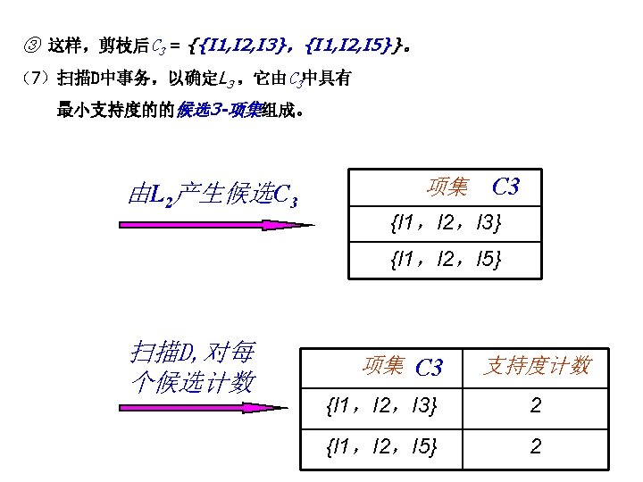
Association Rule Mining Association Rule Mining l Given


 {Milk,")


 – Complete search:")


 Pairs (2 -itemsets) (No need to generate candidates")


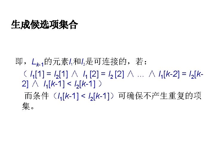
-subsets s of c")


 = {B, C, D, E} Possible")


 TID-list")


 frequent items {f, a,")
 l l l 从FP-tree的频繁项头指针表出发 沿着每个频繁项的指针链,遍历FP-tree 聚集相应频繁项的前缀路径,形成一个条件模式基 {}")

 c: 3")


: minimum support")


-itemset")


 = M(B, A)? Symmetric measures: support, lift,")
: Male Female High 2 3 5")


 u Red cells indicate")


 + -")


- Slides: 116
关联规则挖掘 Association Rule Mining
Association Rule Mining l Given a set of transactions, find rules that will predict the occurrence of an item based on the occurrences of other items in the transaction Market-Basket transactions Example of Association Rules {Diaper} {Beer}, {Milk, Bread} {Eggs, Coke}, {Beer, Bread} {Milk}, Implication means co-occurrence, not causality!
Definition: Frequent Itemset l Itemset – A collection of one or more items u Example: {Milk, Bread, Diaper} – k-itemset u l An itemset that contains k items Support count ( ) – Frequency of occurrence of an itemset – E. g. ({Milk, Bread, Diaper}) = 2 l Support – Fraction of transactions that contain an itemset – E. g. s({Milk, Bread, Diaper}) = 2/5 l Frequent Itemset – An itemset whose support is greater than or equal to a minsup threshold
Definition: Association Rule l Association Rule – An implication expression of the form X Y, where X and Y are itemsets – Example: {Milk, Diaper} {Beer} l Rule Evaluation Metrics – Support (s) u Fraction of transactions that contain both X and Y – Confidence (c) u Measures how often items in Y appear in transactions that contain X Example:
Association Rule Mining Task l Given a set of transactions T, the goal of association rule mining is to find all rules having – support ≥ minsup threshold – confidence ≥ minconf threshold l Brute-force approach: – List all possible association rules – Compute the support and confidence for each rule – Prune rules that fail the minsup and minconf thresholds Computationally prohibitive!
Mining Association Rules Example of Rules: {Milk, Diaper} {Beer} (s=0. 4, c=0. 67) {Milk, Beer} {Diaper} (s=0. 4, c=1. 0) {Diaper, Beer} {Milk} (s=0. 4, c=0. 67) {Beer} {Milk, Diaper} (s=0. 4, c=0. 67) {Diaper} {Milk, Beer} (s=0. 4, c=0. 5) {Milk} {Diaper, Beer} (s=0. 4, c=0. 5) Observations: • All the above rules are binary partitions of the same itemset: {Milk, Diaper, Beer} • Rules originating from the same itemset have identical support but can have different confidence • Thus, we may decouple the support and confidence requirements
Mining Association Rules l Two-step approach: 1. Frequent Itemset Generation – Generate all itemsets whose support minsup 2. Rule Generation – l Generate high confidence rules from each frequent itemset, where each rule is a binary partitioning of a frequent itemset Frequent itemset generation is still computationally expensive
Frequent Itemset Generation Given d items, there are 2 d possible candidate itemsets
Frequent Itemset Generation l Brute-force approach: – Each itemset in the lattice is a candidate frequent itemset – Count the support of each candidate by scanning the database – Match each transaction against every candidate – Complexity ~ O(NMw) => Expensive since M = 2 d !!!
Computational Complexity l Given d unique items: – Total number of itemsets = 2 d – Total number of possible association rules: If d=6, R = 602 rules
Frequent Itemset Generation Strategies l Reduce the number of candidates (M) – Complete search: M=2 d – Use pruning techniques to reduce M l Reduce the number of transactions (N) – Reduce size of N as the size of itemset increases – Used by DHP and vertical-based mining algorithms l Reduce the number of comparisons (NM) – Use efficient data structures to store the candidates or transactions – No need to match every candidate against every transaction
Reducing Number of Candidates l Apriori principle: – If an itemset is frequent, then all of its subsets must also be frequent l Apriori principle holds due to the following property of the support measure: – Support of an itemset never exceeds the support of its subsets – This is known as the anti-monotone property of support
Illustrating Apriori Principle Found to be Infrequent Pruned supersets
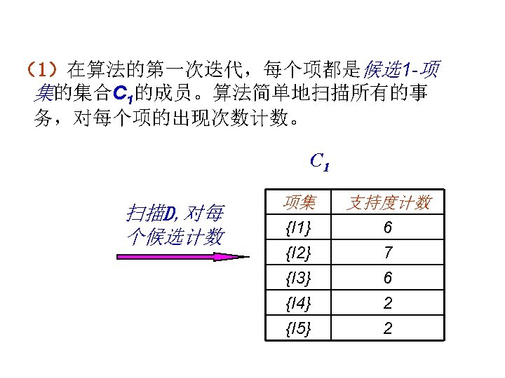
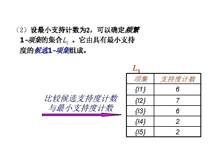
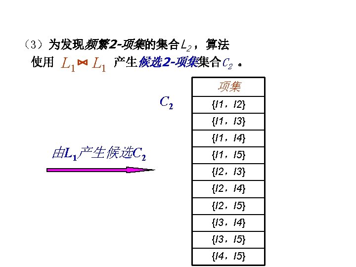
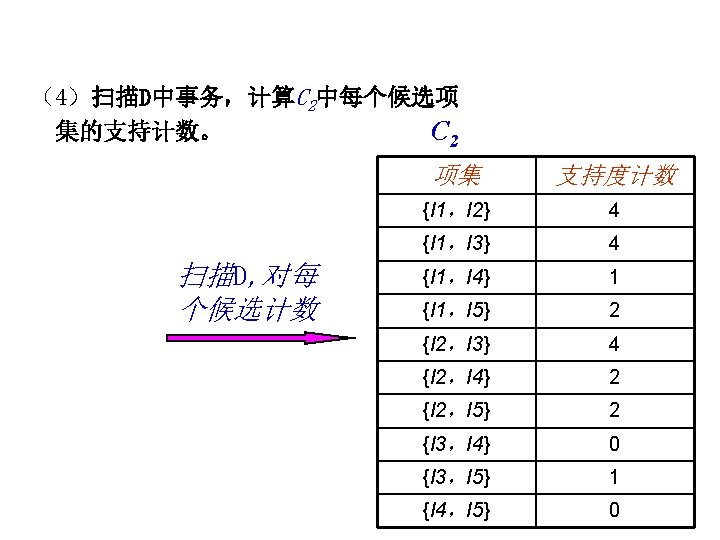
Illustrating Apriori Principle Items (1 -itemsets) Pairs (2 -itemsets) (No need to generate candidates involving Coke or Eggs) Minimum Support = 3 If every subset is considered, 6 C + 6 C = 41 1 2 3 With support-based pruning, 6 + 1 = 13 Triplets (3 -itemsets)
Apriori Algorithm l Method: – Let k=1 – Generate frequent itemsets of length 1 – Repeat until no new frequent itemsets are identified u Generate length (k+1) candidate itemsets from length k frequent itemsets u Prune candidate itemsets containing subsets of length k that are infrequent u Count the support of each candidate by scanning the DB u Eliminate candidates that are infrequent, leaving only those that are frequent
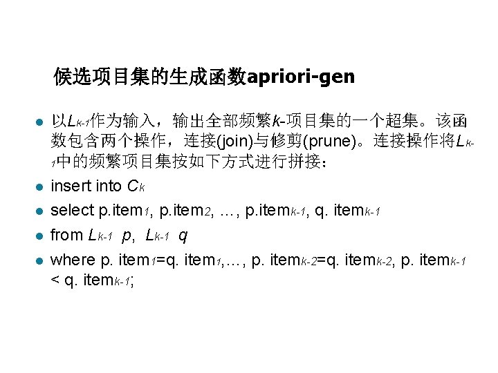
Apriori Algorithm l l l L 1 = {frequent 1 -itemset}; for (k=2; Lk-1 ; k++) do begin Ck = apriori-gen(Lk-1); // 生成大小为k的候选项集合 Ck为大小k的候选项集构成的集合 Lk-1 for all transactions t D do begin Ct = subset(Ck,t); // 事务数据t中包含的候选项集 for all candidates c Ct do c. count ++; end Lk = {c Ck |c. count minsup} end Answer =
修剪操作 l 对Ck中任一候选项集c,若c的某个大小为k-1的子 集不属于Lk-1,则将其从Ck中删除。 forall itemsets c Ck do forall (k-1)-subsets s of c do if (s Lk-1) then delete c from Ck ;
Reducing Number of Comparisons l Candidate counting: – Scan the database of transactions to determine the support of each candidate itemset – To reduce the number of comparisons, store the candidates in a hash structure Instead of matching each transaction against every candidate, match it against candidates contained in the hashed buckets u
Generate Hash Tree Suppose you have 15 candidate itemsets of length 3: {1 4 5}, {1 2 4}, {4 5 7}, {1 2 5}, {4 5 8}, {1 5 9}, {1 3 6}, {2 3 4}, {5 6 7}, {3 4 5}, {3 5 6}, {3 5 7}, {6 8 9}, {3 6 7}, {3 6 8} You need: • Hash function (MOD 3) • Max leaf size: max number of itemsets stored in a leaf node (if number of candidate itemsets exceeds max leaf size, split the node) Hash function 3, 6, 9 1, 4, 7 234 567 345 136 145 2, 5, 8 124 457 125 458 159 356 357 689 367 368
Association Rule Discovery: Hash tree Hash Function 1, 4, 7 Candidate Hash Tree 3, 6, 9 2, 5, 8 234 567 145 136 345 Hash on 1, 4 or 7 124 125 457 458 159 356 357 689 367 368
Association Rule Discovery: Hash tree Hash Function 1, 4, 7 Candidate Hash Tree 3, 6, 9 2, 5, 8 234 567 145 136 345 Hash on 2, 5 or 8 124 125 457 458 159 356 357 689 367 368
Association Rule Discovery: Hash tree Hash Function 1, 4, 7 Candidate Hash Tree 3, 6, 9 2, 5, 8 234 567 145 136 345 Hash on 3, 6 or 9 124 125 457 458 159 356 357 689 367 368
Subset Operation Given a transaction t, what are the possible subsets of size 3?
Subset Operation Using Hash Tree Hash Function 1 2 3 5 6 transaction 1+ 2356 2+ 356 1, 4, 7 3+ 56 234 567 145 136 345 124 457 125 458 159 356 357 689 367 368 2, 5, 8 3, 6, 9
Subset Operation Using Hash Tree Hash Function 1 2 3 5 6 transaction 1+ 2356 2+ 356 1, 4, 7 3+ 56 13+ 56 234 567 15+ 6 145 136 345 124 457 125 458 159 356 357 689 367 368 2, 5, 8 3, 6, 9
Subset Operation Using Hash Tree Hash Function 1 2 3 5 6 transaction 1+ 2356 2+ 356 1, 4, 7 3+ 56 3, 6, 9 2, 5, 8 13+ 56 234 567 15+ 6 145 136 345 124 457 125 458 159 356 357 689 367 368 Match transaction against 11 out of 15 candidates
Factors Affecting Complexity l Choice of minimum support threshold – – l Dimensionality (number of items) of the data set – – l more space is needed to store support count of each item if number of frequent items also increases, both computation and I/O costs may also increase Size of database – l lowering support threshold results in more frequent itemsets this may increase number of candidates and max length of frequent itemsets since Apriori makes multiple passes, run time of algorithm may increase with number of transactions Average transaction width – transaction width increases with denser data sets – This may increase max length of frequent itemsets and traversals of hash tree (number of subsets in a transaction increases with its width)
Apriori. Tid算法
Apriori. Tid算法
Compact Representation of Frequent Itemsets l Some itemsets are redundant because they have identical support as their supersets l Number of frequent itemsets l Need a compact representation
Maximal Frequent Itemset An itemset is maximal frequent if none of its immediate supersets is frequent Maximal Itemsets Infrequent Itemsets Border
Closed Itemset l An itemset is closed if none of its immediate supersets has the same support as the itemset
Maximal vs Closed Itemsets Transaction Ids Not supported by any transactions
Maximal vs Closed Frequent Itemsets Minimum support = 2 Closed but not maximal Closed and maximal # Closed = 9 # Maximal = 4
Maximal vs Closed Itemsets
Alternative Methods for Frequent Itemset Generation l Traversal of Itemset Lattice – General-to-specific vs Specific-to-general
Alternative Methods for Frequent Itemset Generation l Traversal of Itemset Lattice – Equivalent Classes
Alternative Methods for Frequent Itemset Generation l Traversal of Itemset Lattice – Breadth-first vs Depth-first(通常用于发现极大频繁项集)
Alternative Methods for Frequent Itemset Generation l Representation of Database – horizontal vs vertical data layout
Tree Projection Set enumeration tree: Possible Extension: E(A) = {B, C, D, E} Possible Extension: E(ABC) = {D, E}
Tree Projection Items are listed in lexicographic order l Each node P stores the following information: l – – Itemset for node P List of possible lexicographic extensions of P: E(P) Pointer to projected database of its ancestor node Bitvector containing information about which transactions in the projected database contain the itemset (1, 0, 1, 1, 0, 0, …)
Projected Database Original Database: Projected Database for node A: For each transaction T, projected transaction at node A is T E(A)
ECLAT l For each item, store a list of transaction ids (tids) TID-list
ECLAT l Determine support of any k-itemset by intersecting tid-lists of two of its (k-1) subsets. l 3 traversal approaches: – top-down, bottom-up and hybrid l l Advantage: very fast support counting Disadvantage: intermediate tid-lists may become too large for memory
FP-growth Algorithm l Use a compressed representation of the database using an FP-tree l Once an FP-tree has been constructed, it uses a recursive divide-and-conquer approach to mine the frequent itemsets
FP-tree construction null After reading TID=1: A: 1 B: 1 After reading TID=2: A: 1 B: 1 null B: 1 C: 1 D: 1
FP-Tree Construction Transaction Database null B: 3 A: 7 B: 5 Header table C: 1 C: 3 D: 1 D: 1 E: 1 Pointers are used to assist frequent itemset generation
FP-growth C: 1 Conditional Pattern base for D: P = {(A: 1, B: 1, C: 1), (A: 1, B: 1), (A: 1, C: 1), (A: 1), (B: 1, C: 1)} D: 1 Recursively apply FPgrowth on P null A: 7 B: 5 C: 1 C: 3 D: 1 B: 1 D: 1 Frequent Itemsets found (with sup > 1): AD, BD, CD, ACD, BCD
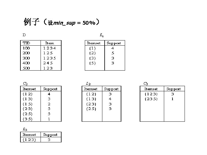
从交易数据库中构造FP-tree TID 100 200 300 400 500 Items bought (ordered) frequent items {f, a, c, d, g, i, m, p} {f, c, a, m, p} {a, b, c, f, l, m, o} {f, c, a, b, m} {b, f, h, j, o} {f, b} {b, c, k, s, p} {c, b, p} {a, f, c, e, l, p, m, n} {f, c, a, m, p} 步骤: Header Table 1. 对DB进行一次扫描, 找出单 个频繁项模式(frequent 1 itemset ); Item frequency head f 4 c 4 a 3 b 3 m 3 p 3 2. 根据频度的降序对频繁项进 行排序; 3. 对DB作第 2次扫描, 构造FPtree。 min_support = 0. 5 {} f: 4 c: 3 c: 1 b: 1 a: 3 b: 1 p: 1 m: 2 b: 1 p: 2 m: 1
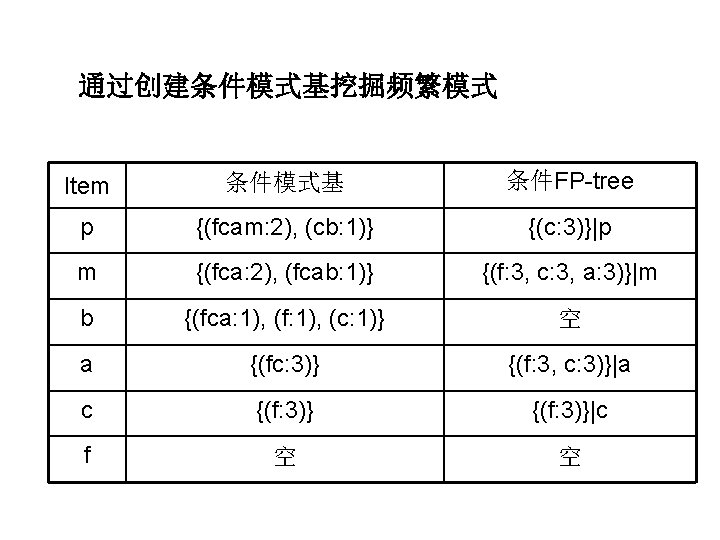
Step 1: 由FP-tree到条件模式基 ( Conditional Pattern Base) l l l 从FP-tree的频繁项头指针表出发 沿着每个频繁项的指针链,遍历FP-tree 聚集相应频繁项的前缀路径,形成一个条件模式基 {} Header Table Item frequency head f 4 c 4 a 3 b 3 m 3 p 3 Conditional pattern bases f: 4 c: 3 c: 1 b: 1 a: 3 b: 1 p: 1 m: 2 b: 1 p: 2 m: 1 item cond. pattern base c f: 3 a fc: 3 b fca: 1, f: 1, c: 1 m fca: 2, fcab: 1 p fcam: 2, cb: 1
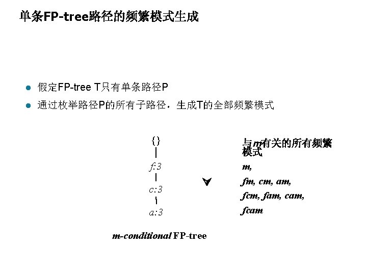
Step 2: 构造条件FP-tree l For each pattern-base – 累加模式基中的每个项的计数 (Accumulate the count for each item in the base) – 为模式基的频繁项构造FP-tree(Construct the FP-tree for the frequent items of the pattern base) {} 项目头指针表 Item frequency head f 4 c 4 a 3 b 3 m 3 p 3 f: 4 c: 3 c: 1 b: 1 p: 1 a: 3 m-conditional pattern base: fca: 2, fcab: 1 {} f: 3 m: 2 b: 1 c: 3 p: 2 m: 1 a: 3 All frequent patterns concerning m m, fm, cm, am, fcm, fam, cam, fcam m-conditional FP-tree
Step 3: 递归挖掘条件FP-tree {} {} Cond. pattern base of “am”: (fc: 3) c: 3 f: 3 am-conditional FP-tree c: 3 a: 3 f: 3 {} Cond. pattern base of “cm”: (f: 3) f: 3 m-conditional FP-tree cm-conditional FP-tree {} Cond. pattern base of “cam”: (f: 3) f: 3 cam-conditional FP-tree
Rule Generation l Given a frequent itemset L, find all non-empty subsets f L such that f L – f satisfies the minimum confidence requirement – If {A, B, C, D} is a frequent itemset, candidate rules: ABC D, A BCD, AB CD, BD AC, l ABD C, B ACD, AC BD, CD AB, ACD B, C ABD, AD BC, BCD A, D ABC BC AD, If |L| = k, then there are 2 k – 2 candidate association rules (ignoring L and L)
Rule Generation l How to efficiently generate rules from frequent itemsets? – In general, confidence does not have an antimonotone property c(ABC D) can be larger or smaller than c(AB D) – But confidence of rules generated from the same itemset has an anti-monotone property – e. g. , L = {A, B, C, D}: c(ABC D) c(AB CD) c(A BCD) Confidence is anti-monotone w. r. t. number of items on the RHS of the rule u
Rule Generation for Apriori Algorithm Lattice of rules Low Confidence Rule Pruned Rules
Rule Generation for Apriori Algorithm l Candidate rule is generated by merging two rules that share the same prefix in the rule consequent l join(CD=>AB, BD=>AC) would produce the candidate rule D => ABC l Prune rule D=>ABC if its subset AD=>BC does not have high confidence
Effect of Support Distribution l Many real data sets have skewed support distribution Support distribution of a retail data set
Effect of Support Distribution l How to set the appropriate minsup threshold? – If minsup is set too high, we could miss itemsets involving interesting rare items (e. g. , expensive products) – If minsup is set too low, it is computationally expensive and the number of itemsets is very large l Using a single minimum support threshold may not be effective
Multiple Minimum Support l How to apply multiple minimum supports? – MS(i): minimum support for item i – e. g. : MS(Milk)=5%, MS(Coke) = 3%, MS(Broccoli)=0. 1%, MS(Salmon)=0. 5% – MS({Milk, Broccoli}) = min (MS(Milk), MS(Broccoli)) = 0. 1% – Challenge: Support is no longer anti-monotone u u Suppose: Support(Milk, Coke) = 1. 5% and Support(Milk, Coke, Broccoli) = 0. 5% {Milk, Coke} is infrequent but {Milk, Coke, Broccoli} is frequent
Multiple Minimum Support
Multiple Minimum Support
Multiple Minimum Support l Order the items according to their minimum support (in ascending order) – e. g. : MS(Milk)=5%, MS(Coke) = 3%, MS(Broccoli)=0. 1%, MS(Salmon)=0. 5% – Ordering: Broccoli, Salmon, Coke, Milk l Need to modify Apriori such that: – L 1 : set of frequent items – F 1 : set of items whose support is MS(1) where MS(1) is mini( MS(i) ) – C 2 : candidate itemsets of size 2 is generated from F 1 instead of L 1
Multiple Minimum Support l Modifications to Apriori: – In traditional Apriori, A candidate (k+1)-itemset is generated by merging two frequent itemsets of size k u The candidate is pruned if it contains any infrequent subsets of size k u – Pruning step has to be modified: Prune only if subset contains the first item u e. g. : Candidate={Broccoli, Coke, Milk} (ordered according to minimum support) u {Broccoli, Coke} and {Broccoli, Milk} are frequent but {Coke, Milk} is infrequent u – Candidate is not pruned because {Coke, Milk} does not contain the first item, i. e. , Broccoli.
Pattern Evaluation l Association rule algorithms tend to produce too many rules – many of them are uninteresting or redundant – Redundant if {A, B, C} {D} and {A, B} {D} have same support & confidence l Interestingness measures can be used to prune/rank the derived patterns l In the original formulation of association rules, support & confidence are the only measures used
Application of Interestingness Measures
Computing Interestingness Measure l Given a rule X Y, information needed to compute rule interestingness can be obtained from a contingency table Contingency table for X Y Y Y X f 11 f 10 f 1+ X f 01 f 00 fo+ f+1 f+0 |T| f 11: support of X and Y f 10: support of X and Y f 01: support of X and Y f 00: support of X and Y Used to define various measures u support, confidence, lift, Gini, J-measure, etc.
Drawback of Confidence Coffee Tea 15 5 20 Tea 75 5 80 90 10 100 Association Rule: Tea Coffee Confidence= P(Coffee|Tea) = 0. 75 but P(Coffee) = 0. 9 Although confidence is high, rule is misleading P(Coffee|Tea) = 0. 9375
Statistical Independence l Population of 1000 students – 600 students know how to swim (S) – 700 students know how to bike (B) – 420 students know how to swim and bike (S, B) – P(S B) = 420/1000 = 0. 42 – P(S) P(B) = 0. 6 0. 7 = 0. 42 – P(S B) = P(S) P(B) => Statistical independence – P(S B) > P(S) P(B) => Positively correlated – P(S B) < P(S) P(B) => Negatively correlated
Statistical-based Measures l Measures that take into account statistical dependence
Example: Lift/Interest Coffee Tea 15 5 20 Tea 75 5 80 90 10 100 Association Rule: Tea Coffee Confidence= P(Coffee|Tea) = 0. 75 but P(Coffee) = 0. 9 Lift = 0. 75/0. 9= 0. 8333 (< 1, therefore is negatively associated)
There are lots of measures proposed in the literature Some measures are good for certain applications, but not for others What criteria should we use to determine whether a measure is good or bad? What about Aprioristyle support based pruning? How does it affect these measures?
Properties of A Good Measure l Piatetsky-Shapiro: 3 properties a good measure M must satisfy: – M(A, B) = 0 if A and B are statistically independent – M(A, B) increase monotonically with P(A, B) when P(A) and P(B) remain unchanged – M(A, B) decreases monotonically with P(A) [or P(B)] when P(A, B) and P(B) [or P(A)] remain unchanged
Comparing Different Measures 10 examples of contingency tables: Rankings of contingency tables using various measures:
Property under Variable Permutation Does M(A, B) = M(B, A)? Symmetric measures: support, lift, collective strength, cosine, Jaccard, etc u Asymmetric measures: u confidence, conviction, Laplace, J-measure, etc
Property under Row/Column Scaling Grade-Gender Example (Mosteller, 1968): Male Female High 2 3 5 Low 1 4 5 3 7 10 Male Female High 4 30 34 Low 2 40 42 6 70 76 2 x 10 x Mosteller: Underlying association should be independent of the relative number of male and female students in the samples
Property under Inversion Operation . . . Transaction 1 Transaction N
Example: -Coefficient l -coefficient is analogous to correlation coefficient for continuous variables Y Y X 60 10 70 X 10 20 30 70 30 100 Y Y X 20 10 30 X 10 60 70 30 70 100 -Coefficient is the same for both tables
Property under Null Addition Invariant measures: u support, cosine, Jaccard, etc Non-invariant measures: u correlation, Gini, mutual information, odds ratio, etc
Different Measures have Different Properties
Support-based Pruning l Most of the association rule mining algorithms use support measure to prune rules and itemsets l Study effect of support pruning on correlation of itemsets – Generate 10000 random contingency tables – Compute support and pairwise correlation for each table – Apply support-based pruning and examine the tables that are removed
Effect of Support-based Pruning
Effect of Support-based Pruning Support-based pruning eliminates mostly negatively correlated itemsets
Effect of Support-based Pruning l Investigate how support-based pruning affects other measures l Steps: – Generate 10000 contingency tables – Rank each table according to the different measures – Compute the pair-wise correlation between the measures
Effect of Support-based Pruning u Without Support Pruning (All Pairs) u Red cells indicate correlation between the pair of measures > 0. 85 u 40. 14% pairs have correlation > 0. 85 Scatter Plot between Correlation & Jaccard Measure
Effect of Support-based Pruning u 0. 5% support 50% Scatter Plot between Correlation & Jaccard Measure: u 61. 45% pairs have correlation > 0. 85
Effect of Support-based Pruning u 0. 5% support 30% Scatter Plot between Correlation & Jaccard Measure u 76. 42% pairs have correlation > 0. 85
Subjective Interestingness Measure l Objective measure: – Rank patterns based on statistics computed from data – e. g. , 21 measures of association (support, confidence, Laplace, Gini, mutual information, Jaccard, etc). l Subjective measure: – Rank patterns according to user’s interpretation u A pattern is subjectively interesting if it contradicts the expectation of a user (Silberschatz & Tuzhilin) u A pattern is subjectively interesting if it is actionable (Silberschatz & Tuzhilin)
Interestingness via Unexpectedness l Need to model expectation of users (domain knowledge) + - Pattern expected to be frequent Pattern expected to be infrequent Pattern found to be infrequent + - + l Expected Patterns Unexpected Patterns Need to combine expectation of users with evidence from data (i. e. , extracted patterns)
Interestingness via Unexpectedness l Web Data – Domain knowledge in the form of site structure – Given an itemset F = {X 1, X 2, …, Xk} (Xi : Web pages) u L: number of links connecting the pages u lfactor = L / (k k-1) u cfactor = 1 (if graph is connected), 0 (disconnected graph) – Structure evidence = cfactor lfactor – Usage evidence – Use Dempster-Shafer theory to combine domain knowledge and evidence from data
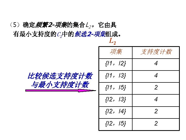
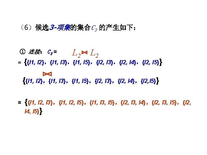
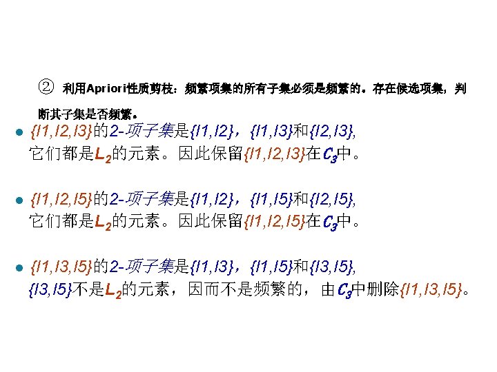
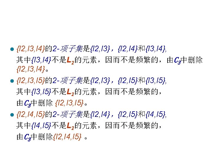
l P 250 2、3、4、9、11