Association Rule Mining CENG 514 Data Mining 20
![Interestingness Measure: Correlation (Lift) • play basketball eat cereal [40%, 66. 7%] is misleading Interestingness Measure: Correlation (Lift) • play basketball eat cereal [40%, 66. 7%] is misleading](https://slidetodoc.com/presentation_image_h2/82b9402041db0b7fffa9db7ee2b1478c/image-51.jpg)
- Slides: 55

Association Rule Mining CENG 514 Data Mining 20. 1. 2022 1

What Is Frequent Pattern Analysis? • Motivation: Finding inherent regularities in data – What products were often purchased together? — Beer and diapers? ! – What are the subsequent purchases after buying a PC? – What kinds of DNA are sensitive to this new drug? • Frequent pattern: a pattern (a set of items, subsequences, substructures, etc. ) that occurs frequently in a data set • First proposed by Agrawal, Imielinski, and Swami [AIS 93] in the context of frequent itemsets and association rule mining 20 January 2022 2

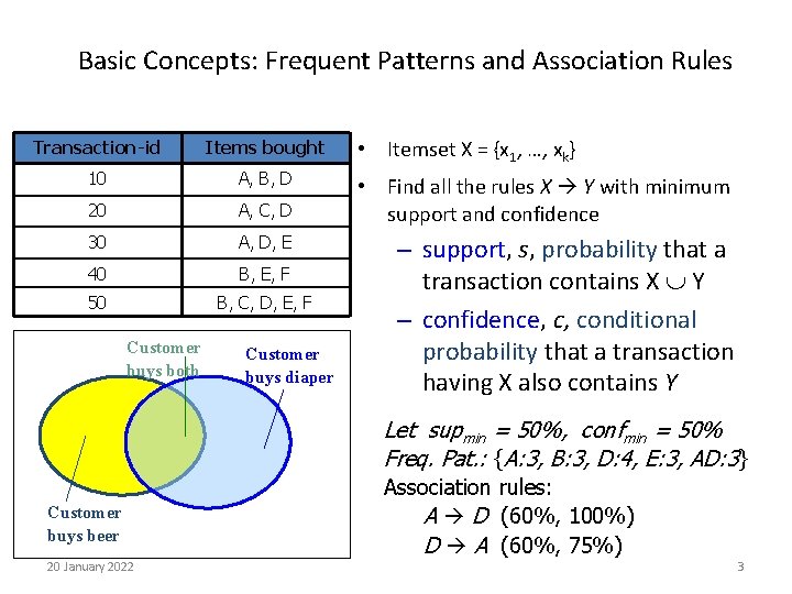
Basic Concepts: Frequent Patterns and Association Rules Transaction-id Items bought 10 A, B, D 20 A, C, D 30 A, D, E 40 B, E, F 50 B, C, D, E, F Customer buys both Customer buys diaper • Itemset X = {x 1, …, xk} • Find all the rules X Y with minimum support and confidence – support, s, probability that a transaction contains X Y – confidence, c, conditional probability that a transaction having X also contains Y Let supmin = 50%, confmin = 50% Freq. Pat. : {A: 3, B: 3, D: 4, E: 3, AD: 3} Customer buys beer 20 January 2022 Association rules: A D (60%, 100%) D A (60%, 75%) 3

Use of Association Rules • Association rules do not represent any sort of causality or correlation between the two itemsets. – X Y does not mean X causes Y, so no Causality – X Y can be different from Y X, unlike correlation • Association rules assist in marketing, targeted advertising, floor planning, inventory control, churning management, homeland security, Basket data analysis, cross-marketing, catalog design, sale campaign analysis, Web log (click stream) analysis, and DNA sequence analysis. Spring 2005 CSE 572, CBS 598 by H. Liu 4

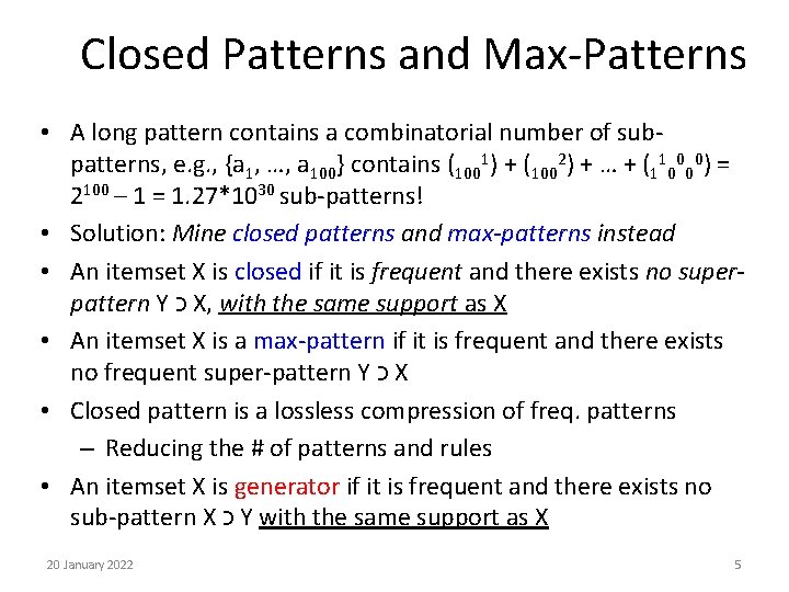
Closed Patterns and Max-Patterns • A long pattern contains a combinatorial number of subpatterns, e. g. , {a 1, …, a 100} contains (1001) + (1002) + … + (110000) = 2100 – 1 = 1. 27*1030 sub-patterns! • Solution: Mine closed patterns and max-patterns instead • An itemset X is closed if it is frequent and there exists no superpattern Y כ X, with the same support as X • An itemset X is a max-pattern if it is frequent and there exists no frequent super-pattern Y כ X • Closed pattern is a lossless compression of freq. patterns – Reducing the # of patterns and rules • An itemset X is generator if it is frequent and there exists no sub-pattern X כ Y with the same support as X 20 January 2022 5

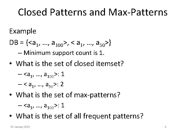
Closed Patterns and Max-Patterns Example DB = {<a 1, …, a 100>, < a 1, …, a 50>} – Minimum support count is 1. • What is the set of closed itemset? – <a 1, …, a 100>: 1 – < a 1, …, a 50>: 2 • What is the set of max-patterns? – <a 1, …, a 100>: 1 • What is the set of all frequent patterns? 20 January 2022 6

Methods for Mining Frequent Patterns • Apriori Rule (The downward closure property) – Any subset of a frequent itemset must be frequent – If {beer, diaper, nuts} is frequent, so is {beer, diaper} – i. e. , every transaction having {beer, diaper, nuts} also contains {beer, diaper} • Basic FIM methods: – Apriori – Freq. pattern growth (Closet. FPgrowth—Han, Pei & Yin @SIGMOD’ 00) – Vertical data format approach (SPADE, CHARM) 20 January 2022 7

Apriori: A Candidate Generation-and-Test Approach • Apriori pruning principle: If there is any itemset which is infrequent, its superset should not be generated/tested! (Agrawal & Srikant @VLDB’ 94, Mannila, et al. @ KDD’ 94) • Method: – Initially, scan DB once to get frequent 1 -itemset – Generate length (k+1) candidate itemsets from length k frequent itemsets – Test the candidates against DB – Terminate when no frequent or candidate set can be generated 20 January 2022 8

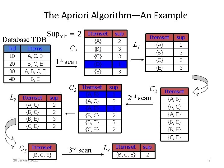
The Apriori Algorithm—An Example Database TDB Tid Items 10 A, C, D 20 B, C, E 30 A, B, C, E 40 B, E Supmin = 2 Itemset {A, C} {B, E} {C, E} sup {A} 2 {B} 3 {C} 3 {D} 1 {E} 3 C 1 1 st scan C 2 L 2 Itemset sup 2 2 3 2 Itemset {A, B} {A, C} {A, E} {B, C} {B, E} {C, E} sup 1 2 3 2 L 1 Itemset sup {A} 2 {B} 3 {C} 3 {E} 3 C 2 2 nd scan Itemset {A, B} {A, C} {A, E} {B, C} {B, E} {C, E} C 3 Itemset {B, C, E} 20 January 2022 3 rd scan L 3 Itemset sup {B, C, E} 2 9

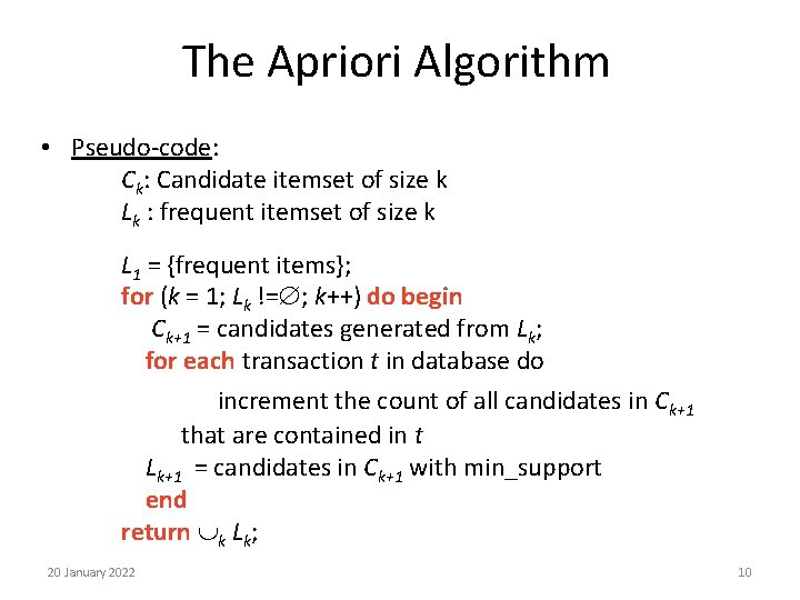
The Apriori Algorithm • Pseudo-code: Ck: Candidate itemset of size k Lk : frequent itemset of size k L 1 = {frequent items}; for (k = 1; Lk != ; k++) do begin Ck+1 = candidates generated from Lk; for each transaction t in database do increment the count of all candidates in Ck+1 that are contained in t Lk+1 = candidates in Ck+1 with min_support end return k Lk; 20 January 2022 10

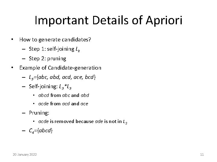
Important Details of Apriori • How to generate candidates? – Step 1: self-joining Lk – Step 2: pruning • Example of Candidate-generation – L 3={abc, abd, ace, bcd} – Self-joining: L 3*L 3 • abcd from abc and abd • acde from acd and ace – Pruning: • acde is removed because ade is not in L 3 – C 4={abcd} 20 January 2022 11

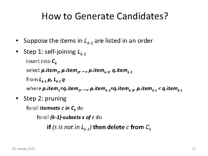
How to Generate Candidates? • Suppose the items in Lk-1 are listed in an order • Step 1: self-joining Lk-1 insert into Ck select p. item 1, p. item 2, …, p. itemk-1, q. itemk-1 from Lk-1 p, Lk-1 q where p. item 1=q. item 1, …, p. itemk-2=q. itemk-2, p. itemk-1 < q. itemk-1 • Step 2: pruning forall itemsets c in Ck do forall (k-1)-subsets s of c do if (s is not in Lk-1) then delete c from Ck 20 January 2022 12

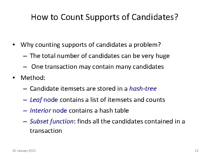
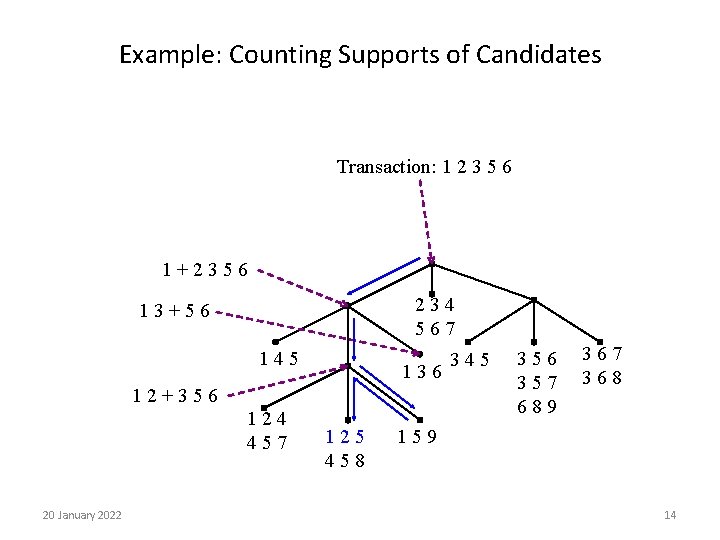
How to Count Supports of Candidates? • Why counting supports of candidates a problem? – The total number of candidates can be very huge – One transaction may contain many candidates • Method: – Candidate itemsets are stored in a hash-tree – Leaf node contains a list of itemsets and counts – Interior node contains a hash table – Subset function: finds all the candidates contained in a transaction 20 January 2022 13

Example: Counting Supports of Candidates Transaction: 1 2 3 5 6 1+2356 234 567 13+56 145 136 12+356 124 457 20 January 2022 125 458 345 356 357 689 367 368 159 14

Challenges of Frequent Pattern Mining • Challenges – Multiple scans of transaction database – Huge number of candidates – Tedious workload of support counting for candidates • Improving Apriori: general ideas – Reduce passes of transaction database scans – Shrink number of candidates – Facilitate support counting of candidates 20 January 2022 15

Partition: Scan Database Only Twice • Any itemset that is potentially frequent in DB must be frequent in at least one of the partitions of DB – Scan 1: partition database and find local frequent patterns – Scan 2: consolidate global frequent patterns • A. Savasere, E. Omiecinski, and S. Navathe. An efficient algorithm for mining association in large databases. In VLDB’ 95 20 January 2022 16

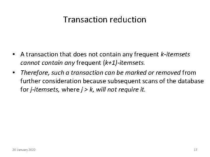
Transaction reduction • A transaction that does not contain any frequent k-itemsets cannot contain any frequent (k+1)-itemsets. • Therefore, such a transaction can be marked or removed from further consideration because subsequent scans of the database for j-itemsets, where j > k, will not require it. 20 January 2022 17

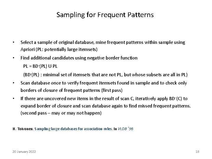
Sampling for Frequent Patterns • Select a sample of original database, mine frequent patterns within sample using Apriori (PL: potentially large itemsets) • Find additional candidates using negative border function PL = BD-(PL) U PL (BD-(PL) : minimal set of itemsets that are not PL, but whose subsets are all in PL) • Scan database once to verify frequent itemsets found in sample and to check only borders of closure of frequent patterns (first pass) • If there are uncovered new items in the result of scan C, iteratively apply BD -(C) to expand border of closure and scan database again to find missed frequent patterns. (second pass – may or may not happen) H. Toivonen. Sampling large databases for association rules. In VLDB’ 96 20 January 2022 18

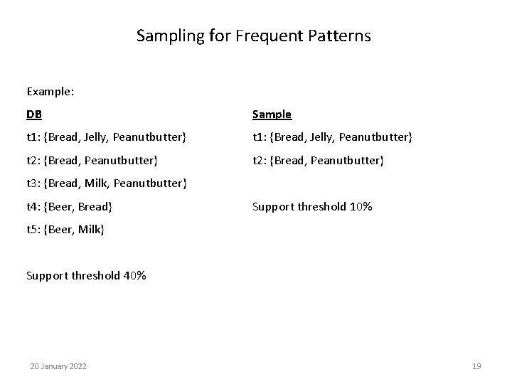
Sampling for Frequent Patterns Example: DB Sample t 1: {Bread, Jelly, Peanutbutter} t 2: {Bread, Peanutbutter} t 3: {Bread, Milk, Peanutbutter} t 4: {Beer, Bread} Support threshold 10% t 5: {Beer, Milk} Support threshold 40% 20 January 2022 19

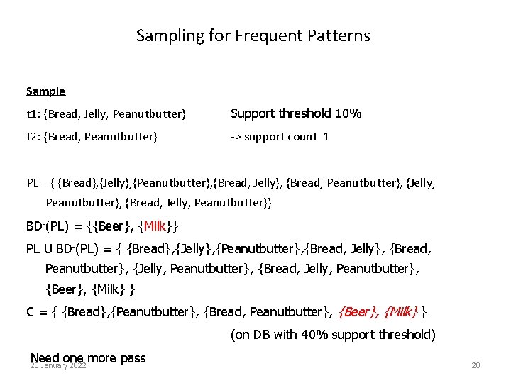
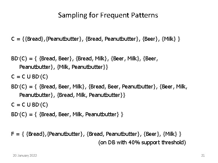
Sampling for Frequent Patterns Sample t 1: {Bread, Jelly, Peanutbutter} Support threshold 10% t 2: {Bread, Peanutbutter} -> support count 1 PL = { {Bread}, {Jelly}, {Peanutbutter}, {Bread, Jelly}, {Bread, Peanutbutter}, {Jelly, Peanutbutter}, {Bread, Jelly, Peanutbutter}} BD-(PL) = {{Beer}, {Milk}} PL U BD-(PL) = { {Bread}, {Jelly}, {Peanutbutter}, {Bread, Jelly}, {Bread, Peanutbutter}, {Jelly, Peanutbutter}, {Bread, Jelly, Peanutbutter}, {Beer}, {Milk} } C = { {Bread}, {Peanutbutter}, {Bread, Peanutbutter}, {Beer}, {Milk} } (on DB with 40% support threshold) Need one more pass 20 January 2022 20

Sampling for Frequent Patterns C = {{Bread}, {Peanutbutter}, {Bread, Peanutbutter}, {Beer}, {Milk} } BD-(C) = { {Bread, Beer}, {Bread, Milk}, {Beer, Peanutbutter}, {Milk, Peanutbutter}} C = C U BD-(C) = { {Bread, Beer, Milk}, {Bread, Beer, Peanutbutter}, {Beer, Milk, Peanutbutter}, {Bread, Milk, Peanutbutter}} C = C U BD-(C) = { {Bread, Beer, Milk, Peanutbutter} } F = { {Bread}, {Peanutbutter}, {Bread, Peanutbutter}, {Beer}, {Milk} } (on DB with 40% support threshold) 20 January 2022 21

Mining Frequent Patterns Without Candidate Generation • Build a compact representation so that no need scan db several times • Find frequent itemsets in a recursive way 20 January 2022 22

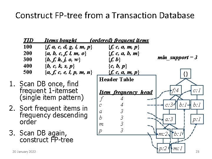
Construct FP-tree from a Transaction Database TID 100 200 300 400 500 Items bought (ordered) frequent items {f, a, c, d, g, i, m, p} {f, c, a, m, p} {a, b, c, f, l, m, o} {f, c, a, b, m} {b, f, h, j, o, w} {f, b} {b, c, k, s, p} {c, b, p} {a, f, c, e, l, p, m, n} {f, c, a, m, p} Header Table 1. Scan DB once, find frequent 1 -itemset (single item pattern) 2. Sort frequent items in frequency descending order 3. Scan DB again, construct FP-tree 20 January 2022 Item frequency head f 4 c 4 a 3 b 3 m 3 p 3 min_support = 3 {} f: 4 c: 3 c: 1 b: 1 a: 3 b: 1 p: 1 m: 2 b: 1 p: 2 m: 1 23

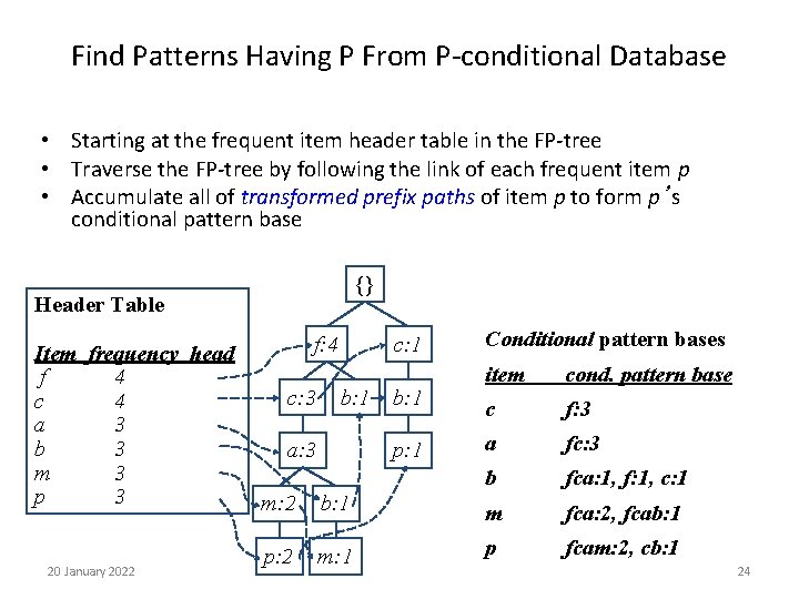
Find Patterns Having P From P-conditional Database • Starting at the frequent item header table in the FP-tree • Traverse the FP-tree by following the link of each frequent item p • Accumulate all of transformed prefix paths of item p to form p’s conditional pattern base {} Header Table Item frequency head f 4 c 4 a 3 b 3 m 3 p 3 20 January 2022 f: 4 c: 3 c: 1 b: 1 a: 3 b: 1 p: 1 Conditional pattern bases item cond. pattern base c f: 3 a fc: 3 b fca: 1, f: 1, c: 1 m: 2 b: 1 m fca: 2, fcab: 1 p: 2 m: 1 p fcam: 2, cb: 1 24

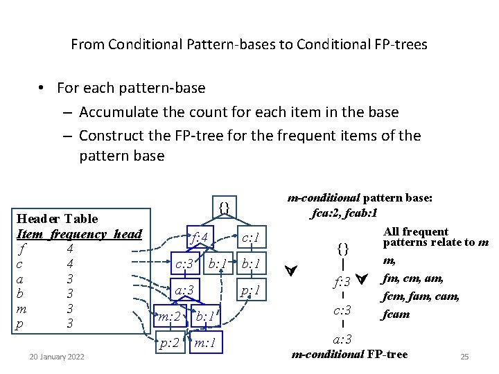
From Conditional Pattern-bases to Conditional FP-trees • For each pattern-base – Accumulate the count for each item in the base – Construct the FP-tree for the frequent items of the pattern base Header Table Item frequency head f 4 c 4 a 3 b 3 m 3 p 3 20 January 2022 m-conditional pattern base: fca: 2, fcab: 1 {} f: 4 c: 3 c: 1 b: 1 a: 3 b: 1 p: 1 {} f: 3 m: 2 b: 1 c: 3 p: 2 m: 1 a: 3 All frequent patterns relate to m m, fm, cm, am, fcm, fam, cam, fcam m-conditional FP-tree 25

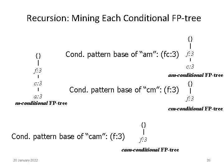
Recursion: Mining Each Conditional FP-tree {} {} Cond. pattern base of “am”: (fc: 3) c: 3 f: 3 c: 3 a: 3 f: 3 am-conditional FP-tree Cond. pattern base of “cm”: (f: 3) {} f: 3 m-conditional FP-tree cm-conditional FP-tree {} Cond. pattern base of “cam”: (f: 3) f: 3 cam-conditional FP-tree 20 January 2022 26

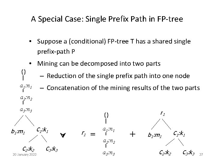
A Special Case: Single Prefix Path in FP-tree • Suppose a (conditional) FP-tree T has a shared single prefix-path P • Mining can be decomposed into two parts {} – Reduction of the single prefix path into one node a 1: n 1 – Concatenation of the mining results of the two parts a 2: n 2 a 3: n 3 b 1: m 1 C 2: k 2 r 1 {} C 1: k 1 20 January 2022 C 3: k 3 r 1 = a 1: n 1 a 2: n 2 a 3: n 3 + b 1: m 1 C 2: k 2 C 1: k 1 C 3: k 3 27

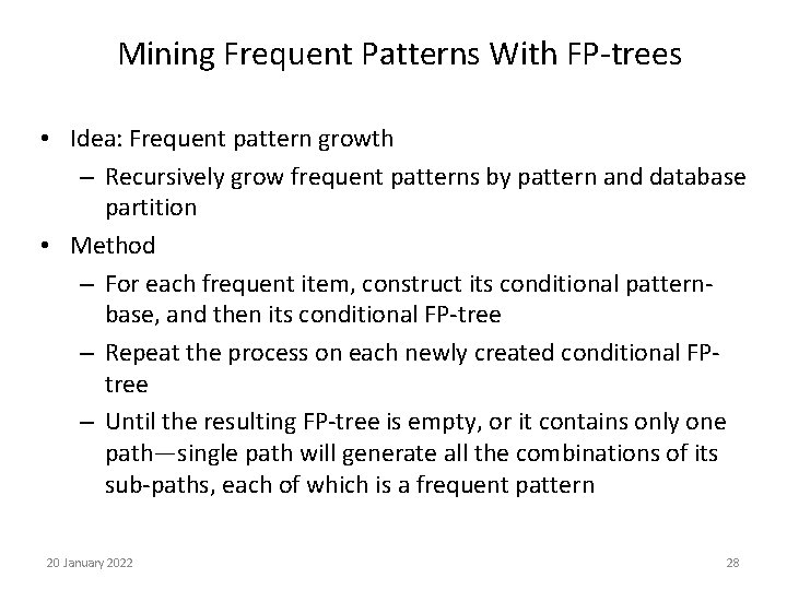
Mining Frequent Patterns With FP-trees • Idea: Frequent pattern growth – Recursively grow frequent patterns by pattern and database partition • Method – For each frequent item, construct its conditional patternbase, and then its conditional FP-tree – Repeat the process on each newly created conditional FPtree – Until the resulting FP-tree is empty, or it contains only one path—single path will generate all the combinations of its sub-paths, each of which is a frequent pattern 20 January 2022 28

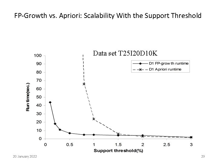
FP-Growth vs. Apriori: Scalability With the Support Threshold Data set T 25 I 20 D 10 K 20 January 2022 29

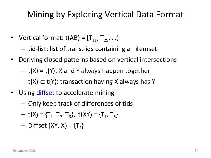
Mining by Exploring Vertical Data Format • Vertical format: t(AB) = {T 11, T 25, …} – tid-list: list of trans. -ids containing an itemset • Deriving closed patterns based on vertical intersections – t(X) = t(Y): X and Y always happen together – t(X) t(Y): transaction having X always has Y • Using diffset to accelerate mining – Only keep track of differences of tids – t(X) = {T 1, T 2, T 3}, t(XY) = {T 1, T 3} – Diffset (XY, X) = {T 2} 20 January 2022 30

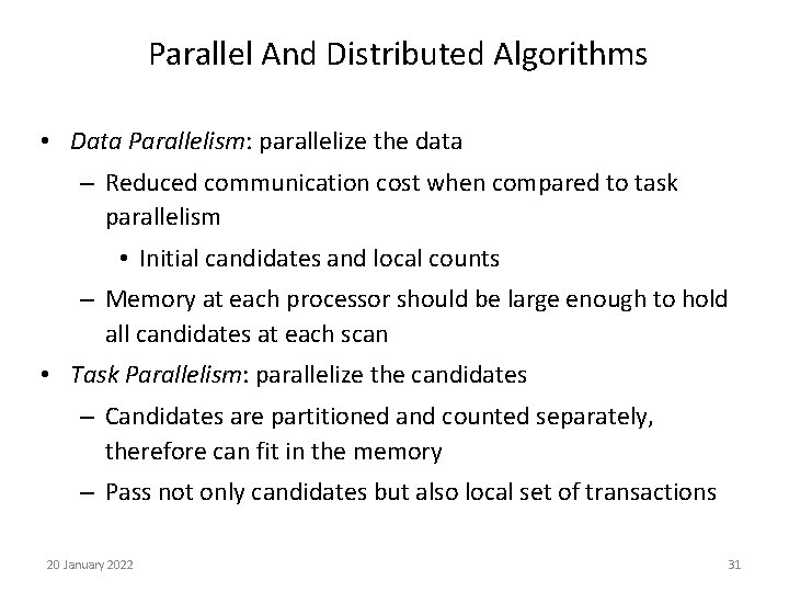
Parallel And Distributed Algorithms • Data Parallelism: parallelize the data – Reduced communication cost when compared to task parallelism • Initial candidates and local counts – Memory at each processor should be large enough to hold all candidates at each scan • Task Parallelism: parallelize the candidates – Candidates are partitioned and counted separately, therefore can fit in the memory – Pass not only candidates but also local set of transactions 20 January 2022 31

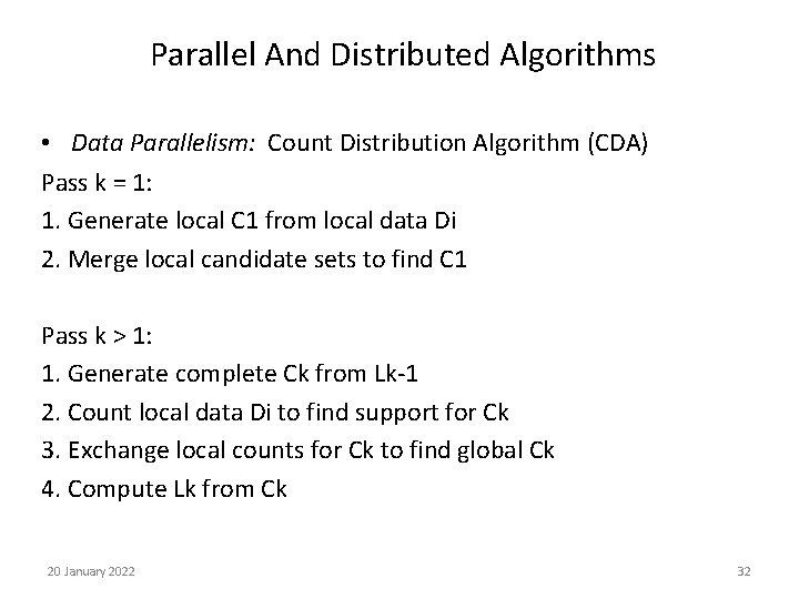
Parallel And Distributed Algorithms • Data Parallelism: Count Distribution Algorithm (CDA) Pass k = 1: 1. Generate local C 1 from local data Di 2. Merge local candidate sets to find C 1 Pass k > 1: 1. Generate complete Ck from Lk-1 2. Count local data Di to find support for Ck 3. Exchange local counts for Ck to find global Ck 4. Compute Lk from Ck 20 January 2022 32

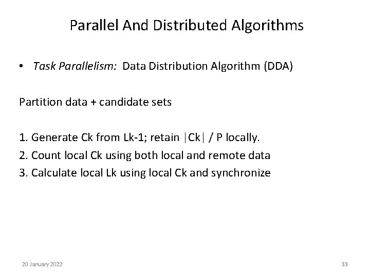
Parallel And Distributed Algorithms • Task Parallelism: Data Distribution Algorithm (DDA) Partition data + candidate sets 1. Generate Ck from Lk-1; retain |Ck| / P locally. 2. Count local Ck using both local and remote data 3. Calculate local Lk using local Ck and synchronize 20 January 2022 33

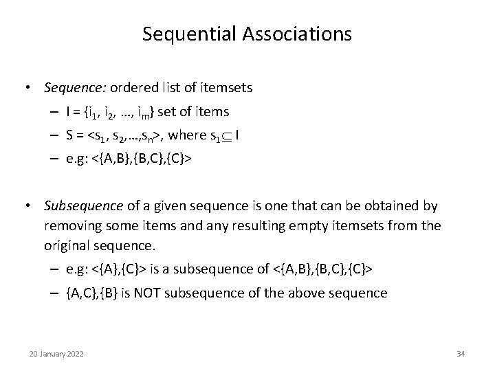
Sequential Associations • Sequence: ordered list of itemsets – I = {i 1, i 2, …, im} set of items – S = <s 1, s 2, …, sn>, where s 1 I – e. g: <{A, B}, {B, C}, {C}> • Subsequence of a given sequence is one that can be obtained by removing some items and any resulting empty itemsets from the original sequence. – e. g: <{A}, {C}> is a subsequence of <{A, B}, {B, C}, {C}> – {A, C}, {B} is NOT subsequence of the above sequence 20 January 2022 34

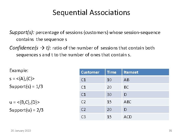
Sequential Associations Support(s): percentage of sessions (customers) whose session-sequence contains the sequence s Confidence(s → t): ratio of the number of sessions that contain both sequences s and t to the number of ones that contain s. Example: Customer Time Itemset s = <{A}, {C}> C 1 10 AB Support(s) = 1/3 C 1 20 BC C 1 30 D u = <{B, C}, {D}> C 2 15 ABC Support(u) = 2/3 C 2 20 D C 3 15 ACD 20 January 2022 35

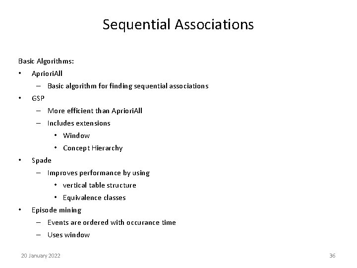
Sequential Associations Basic Algorithms: • Apriori. All – Basic algorithm for finding sequential associations • GSP – More efficient than Apriori. All – Includes extensions • Window • Concept Hierarchy • Spade – Improves performance by using • vertical table structure • Equivalence classes • Episode mining – Events are ordered with occurance time – Uses window 20 January 2022 36

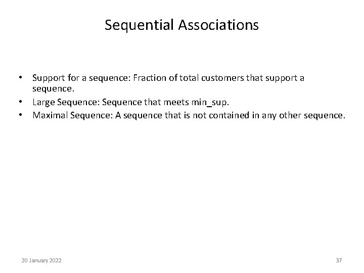
Sequential Associations • Support for a sequence: Fraction of total customers that support a sequence. • Large Sequence: Sequence that meets min_sup. • Maximal Sequence: A sequence that is not contained in any other sequence. 20 January 2022 37

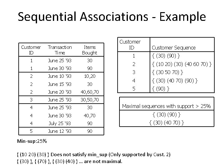
Sequential Associations - Example Customer ID Transaction Time Items Bought 1 June 25 '93 30 1 June 30 '93 90 2 June 10 '93 10, 20 2 June 15 '93 30 2 June 20 '93 40, 60, 70 3 June 25 '93 30, 50, 70 4 June 25 '93 30 Maximal sequences with support > 25% 4 June 30 '93 40, 70 { (30) (90) } 4 July 25 '93 90 { (30) (40 70) } 5 June 12 '93 90 Customer Sequence 1 { (30) (90) } 2 { (10 20) (30) (40 60 70) } 3 { (30 50 70) } 4 { (30) (40 70) (90) } 5 { (90) } Min-sup: 25% { (10 20) (30) } Does not satisfy min_sup (Only supported by Cust. 2) { (30) }, { (70) }, { (30) (40) } … are not maximal.

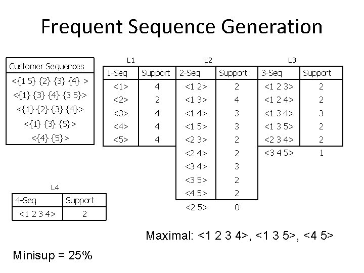
Frequent Sequence Generation Customer Sequences <{1 5} {2} {3} {4} > L 2 L 1 1 -Seq Support 2 -Seq L 3 Support 3 -Seq Support <1> 4 <1 2> 2 <1 2 3> 2 <2> 2 <1 3> 4 <1 2 4> 2 <{1} {2} {3} {4}> <3> 4 <1 4> 3 <1 3 4> 3 <{1} {3} {5}> <4> 4 <1 5> 3 <1 3 5> 2 <{4} {5}> <5> 4 <2 3> 2 <2 3 4> 2 <2 4> 2 <3 4 5> 1 <3 4> 3 <3 5> 2 <4 5> 2 <2 5> 0 <{1} {3} {4} {3 5}> L 4 4 -Seq <1 2 3 4> Support 2 Maximal: <1 2 3 4>, <1 3 5>, <4 5> Minisup = 25%

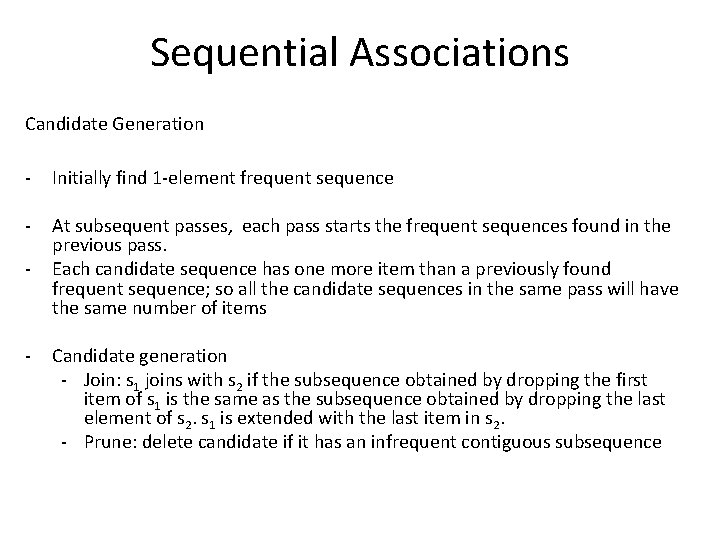
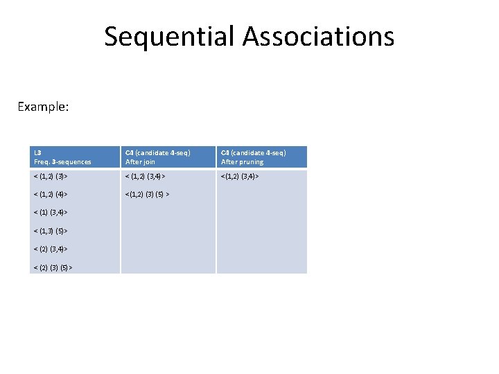
Sequential Associations Candidate Generation - Initially find 1 -element frequent sequence - At subsequent passes, each pass starts the frequent sequences found in the previous pass. Each candidate sequence has one more item than a previously found frequent sequence; so all the candidate sequences in the same pass will have the same number of items - - Candidate generation - Join: s 1 joins with s 2 if the subsequence obtained by dropping the first item of s 1 is the same as the subsequence obtained by dropping the last element of s 2. s 1 is extended with the last item in s 2. - Prune: delete candidate if it has an infrequent contiguous subsequence

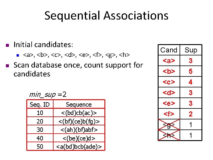
Sequential Associations n Initial candidates: n n <a>, <b>, <c>, <d>, <e>, <f>, <g>, <h> Scan database once, count support for candidates min_sup =2 Seq. ID 10 20 30 40 50 Sequence <(bd)cb(ac)> <(bf)(ce)b(fg)> <(ah)(bf)abf> <(be)(ce)d> <a(bd)bcb(ade)> Cand Sup <a> 3 <b> 5 <c> 4 <d> <e> <f> <g> <h> 3 3 2 1 1

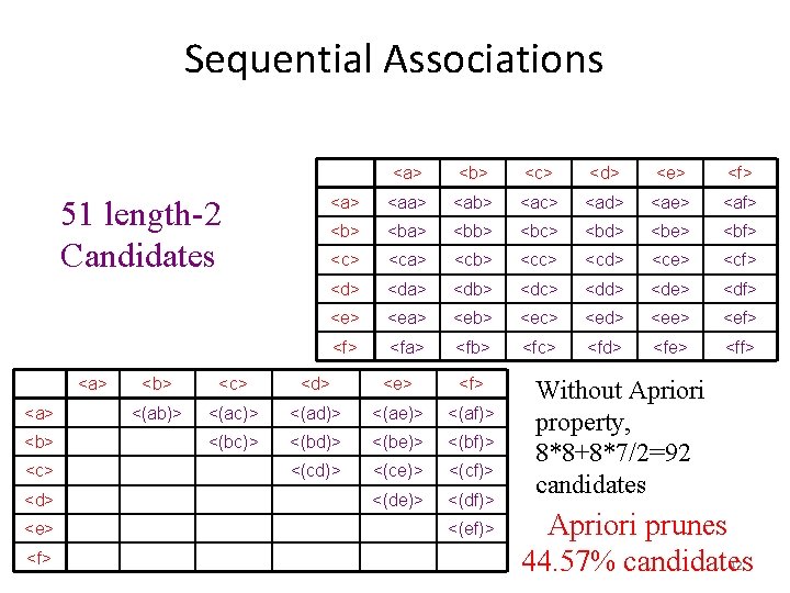
Sequential Associations 51 length-2 Candidates <a> <b> <c> <d> <e> <f> <a> <aa> <ab> <ac> <ad> <ae> <af> <ba> <bb> <bc> <bd> <be> <bf> <ca> <cb> <cc> <cd> <ce> <cf> <da> <db> <dc> <dd> <de> <df> <ea> <eb> <ec> <ed> <ee> <ef> <fa> <fb> <fc> <fd> <fe> <ff> <b> <c> <d> <e> <f> <(ab)> <(ac)> <(ad)> <(ae)> <(af)> <(bc)> <(bd)> <(be)> <(bf)> <(cd)> <(ce)> <(cf)> <(de)> <(df)> <(ef)> Without Apriori property, 8*8+8*7/2=92 candidates Apriori prunes 42 44. 57% candidates

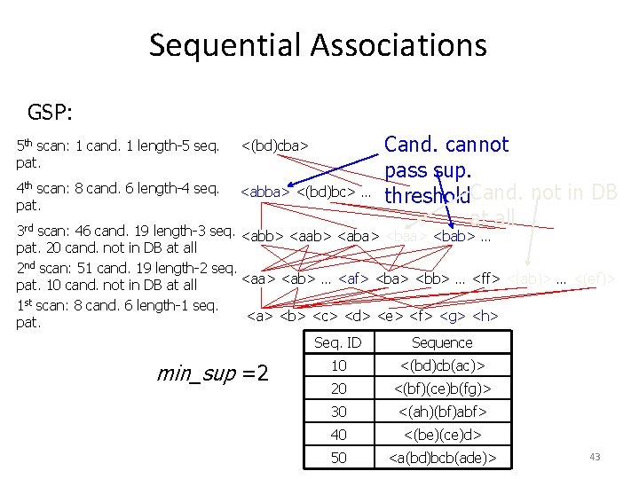
Sequential Associations GSP: 5 th scan: 1 cand. 1 length-5 seq. pat. <(bd)cba> 4 th scan: 8 cand. 6 length-4 seq. pat. <abba> <(bd)bc> … Cand. cannot pass sup. threshold. Cand. not in DB at all 3 rd scan: 46 cand. 19 length-3 seq. <abb> <aab> <aba> <bab> … pat. 20 cand. not in DB at all 2 nd scan: 51 cand. 19 length-2 seq. <aa> <ab> … <af> <ba> <bb> … <ff> <(ab)> … <(ef)> pat. 10 cand. not in DB at all 1 st scan: 8 cand. 6 length-1 seq. <a> <b> <c> <d> <e> <f> <g> <h> pat. Seq. ID Sequence min_sup =2 10 <(bd)cb(ac)> 20 <(bf)(ce)b(fg)> 30 <(ah)(bf)abf> 40 <(be)(ce)d> 50 <a(bd)bcb(ade)> 43

Sequential Associations Example: L 3 Freq. 3 -sequences C 4 (candidate 4 -seq) After join C 4 (candidate 4 -seq) After pruning < (1, 2) (3)> < (1, 2) (3, 4)> < (1, 2) (4)> <(1, 2) (3) (5) > < (1) (3, 4)> < (1, 3) (5)> < (2) (3, 4)> < (2) (3) (5)>

Sequential Associations Extended features – Concept hierarchies (taxonomies) – Sliding window – Time constraints

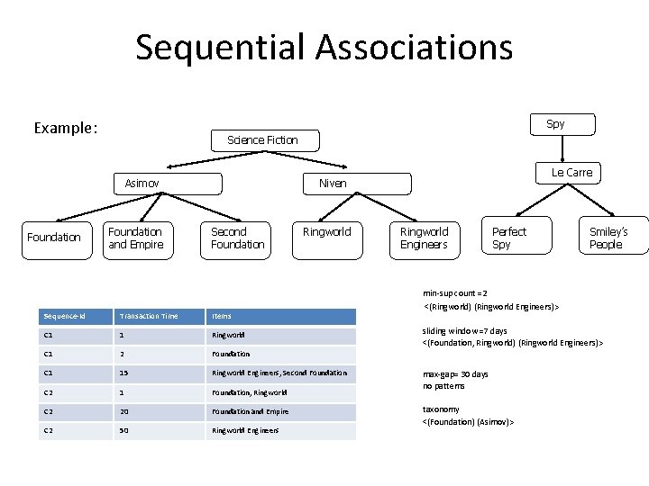
Sequential Associations Spy Example: Science Fiction Asimov Foundation and Empire Le Carre Niven Second Foundation Ringworld Engineers Perfect Spy Smiley’s People min-sup count =2 Sequence-Id Transaction Time Items C 1 1 Ringworld C 1 2 Foundation C 1 15 Ringworld Engineers, Second Foundation C 2 1 Foundation, Ringworld C 2 20 Foundation and Empire C 2 50 Ringworld Engineers <(Ringworld) (Ringworld Engineers)> sliding window =7 days <(Foundation, Ringworld) (Ringworld Engineers)> max-gap= 30 days no patterns taxonomy <(Foundation) (Asimov)>

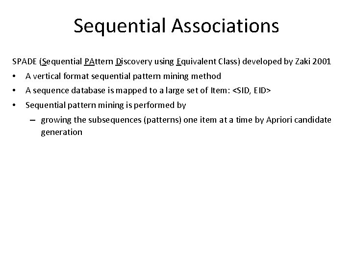
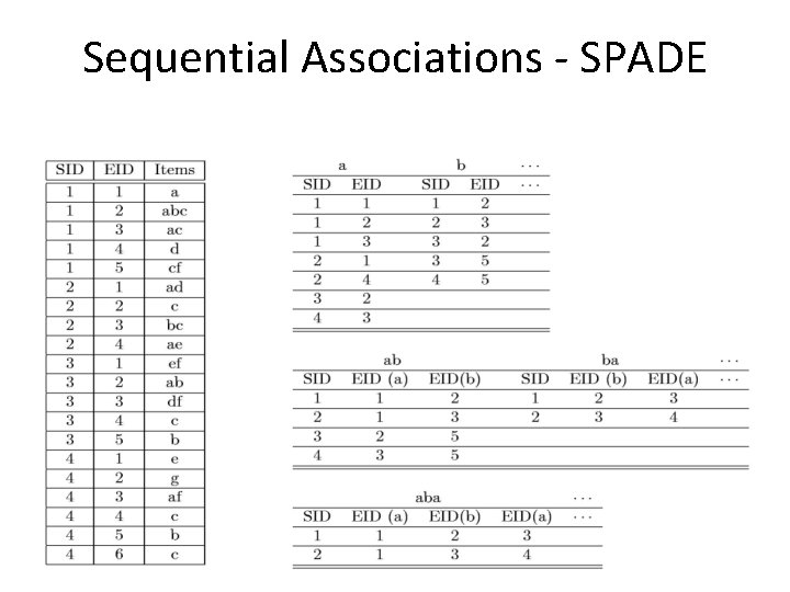
Sequential Associations SPADE (Sequential PAttern Discovery using Equivalent Class) developed by Zaki 2001 • A vertical format sequential pattern mining method • A sequence database is mapped to a large set of Item: <SID, EID> • Sequential pattern mining is performed by – growing the subsequences (patterns) one item at a time by Apriori candidate generation

Sequential Associations - SPADE

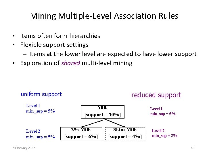
Mining Multiple-Level Association Rules • Items often form hierarchies • Flexible support settings – Items at the lower level are expected to have lower support • Exploration of shared multi-level mining reduced support uniform support Level 1 min_sup = 5% Level 2 min_sup = 5% 20 January 2022 Milk [support = 10%] 2% Milk [support = 6%] Skim Milk [support = 4%] Level 1 min_sup = 5% Level 2 min_sup = 3% 49

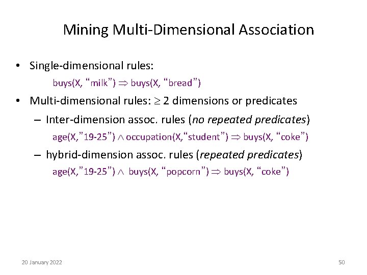
Mining Multi-Dimensional Association • Single-dimensional rules: buys(X, “milk”) buys(X, “bread”) • Multi-dimensional rules: 2 dimensions or predicates – Inter-dimension assoc. rules (no repeated predicates) age(X, ” 19 -25”) occupation(X, “student”) buys(X, “coke”) – hybrid-dimension assoc. rules (repeated predicates) age(X, ” 19 -25”) buys(X, “popcorn”) buys(X, “coke”) 20 January 2022 50
![Interestingness Measure Correlation Lift play basketball eat cereal 40 66 7 is misleading Interestingness Measure: Correlation (Lift) • play basketball eat cereal [40%, 66. 7%] is misleading](https://slidetodoc.com/presentation_image_h2/82b9402041db0b7fffa9db7ee2b1478c/image-51.jpg)
Interestingness Measure: Correlation (Lift) • play basketball eat cereal [40%, 66. 7%] is misleading – The overall % of students eating cereal is 75% > 66. 7%. • play basketball not eat cereal [20%, 33. 3%] is more accurate, although with lower support and confidence • Measure of dependent/correlated events: lift (also called correlation, interest) 20 January 2022 Basketball Not basketball Sum (row) Cereal 2000 1750 3750 Not cereal 1000 250 1250 Sum(col. ) 3000 2000 51

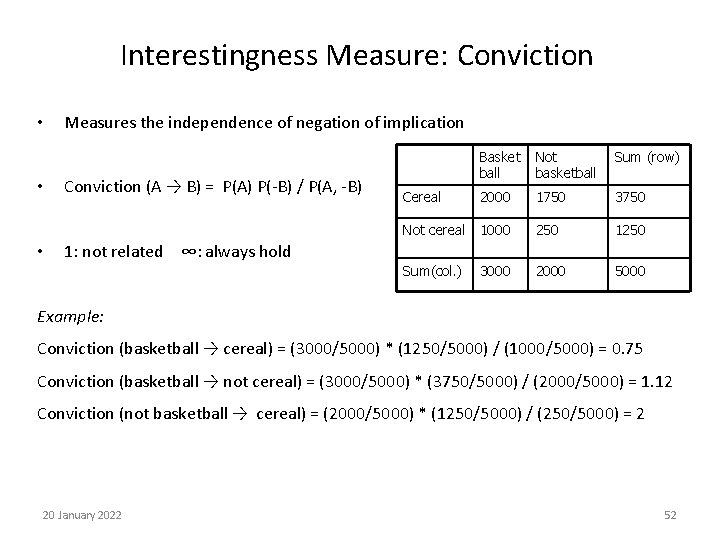
Interestingness Measure: Conviction • • • Measures the independence of negation of implication Conviction (A → B) = P(A) P(-B) / P(A, -B) Basket ball Not basketball Sum (row) 2000 1750 3750 Not cereal 1000 250 1250 Sum(col. ) 2000 5000 Cereal 1: not related ∞: always hold 3000 Example: Conviction (basketball → cereal) = (3000/5000) * (1250/5000) / (1000/5000) = 0. 75 Conviction (basketball → not cereal) = (3000/5000) * (3750/5000) / (2000/5000) = 1. 12 Conviction (not basketball → cereal) = (2000/5000) * (1250/5000) / (250/5000) = 2 20 January 2022 52

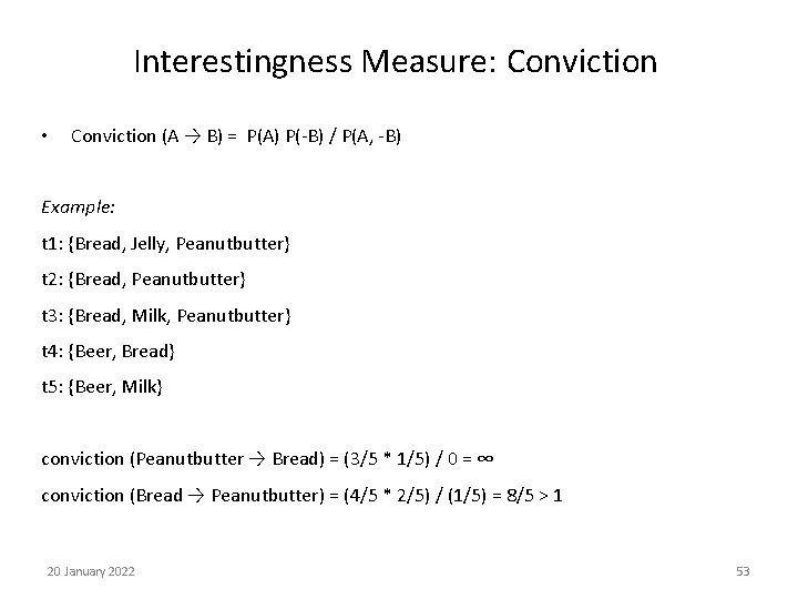
Interestingness Measure: Conviction • Conviction (A → B) = P(A) P(-B) / P(A, -B) Example: t 1: {Bread, Jelly, Peanutbutter} t 2: {Bread, Peanutbutter} t 3: {Bread, Milk, Peanutbutter} t 4: {Beer, Bread} t 5: {Beer, Milk} conviction (Peanutbutter → Bread) = (3/5 * 1/5) / 0 = ∞ conviction (Bread → Peanutbutter) = (4/5 * 2/5) / (1/5) = 8/5 > 1 20 January 2022 53

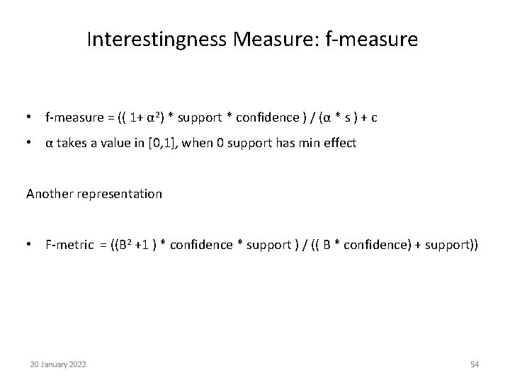
Interestingness Measure: f-measure • f-measure = (( 1+ α 2) * support * confidence ) / (α * s ) + c • α takes a value in [0, 1], when 0 support has min effect Another representation • F-metric = ((B 2 +1 ) * confidence * support ) / (( B * confidence) + support)) 20 January 2022 54

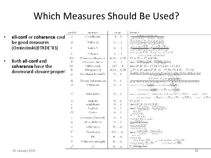
Which Measures Should Be Used? • all-conf or coherence could be good measures (Omiecinski@TKDE’ 03) • Both all-conf and coherence have the downward closure property 20 January 2022 55