More on Rankings Queryindependent LAR Have an apriori

More on Rankings

Query-independent LAR • Have an a-priori ordering of the web pages • Q: Set of pages that contain the keywords in the query q • Present the pages in Q ordered according to order π • What are the advantages of such an approach?

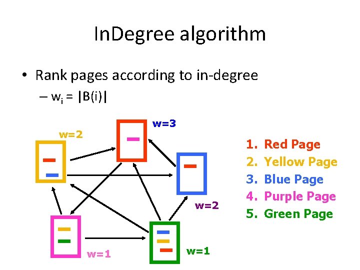
In. Degree algorithm • Rank pages according to in-degree – wi = |B(i)| w=3 w=2 w=1 1. 2. 3. 4. 5. Red Page Yellow Page Blue Page Purple Page Green Page

Page. Rank algorithm [BP 98] • Good authorities should be pointed by good authorities • Random walk on the web graph – pick a page at random – with probability 1 - α jump to a random page – with probability α follow a random outgoing link • Rank according to the stationary distribution • 1. 2. 3. 4. 5. Red Page Purple Page Yellow Page Blue Page Green Page

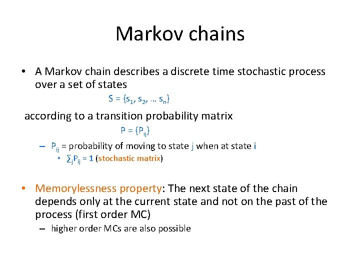
Markov chains • A Markov chain describes a discrete time stochastic process over a set of states S = {s 1, s 2, … sn} according to a transition probability matrix P = {Pij} – Pij = probability of moving to state j when at state i • ∑j. Pij = 1 (stochastic matrix) • Memorylessness property: The next state of the chain depends only at the current state and not on the past of the process (first order MC) – higher order MCs are also possible

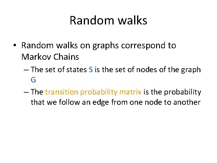
Random walks • Random walks on graphs correspond to Markov Chains – The set of states S is the set of nodes of the graph G – The transition probability matrix is the probability that we follow an edge from one node to another

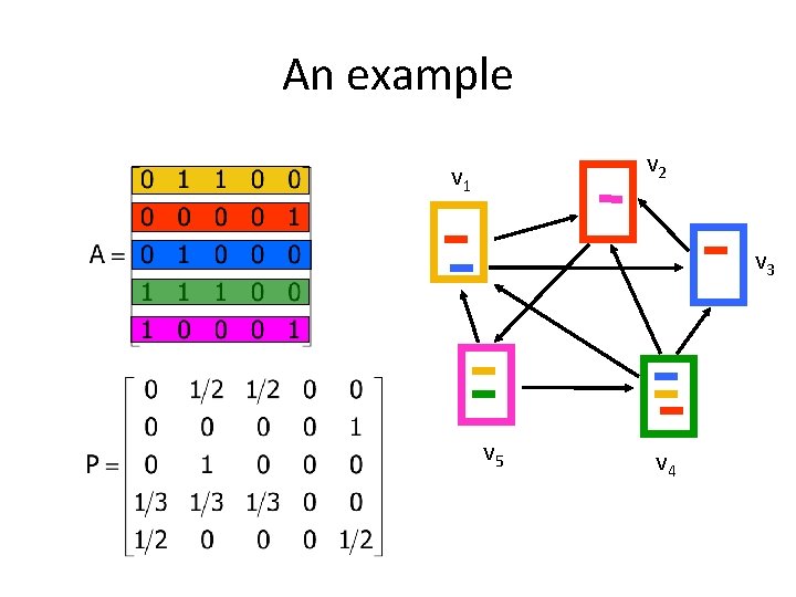
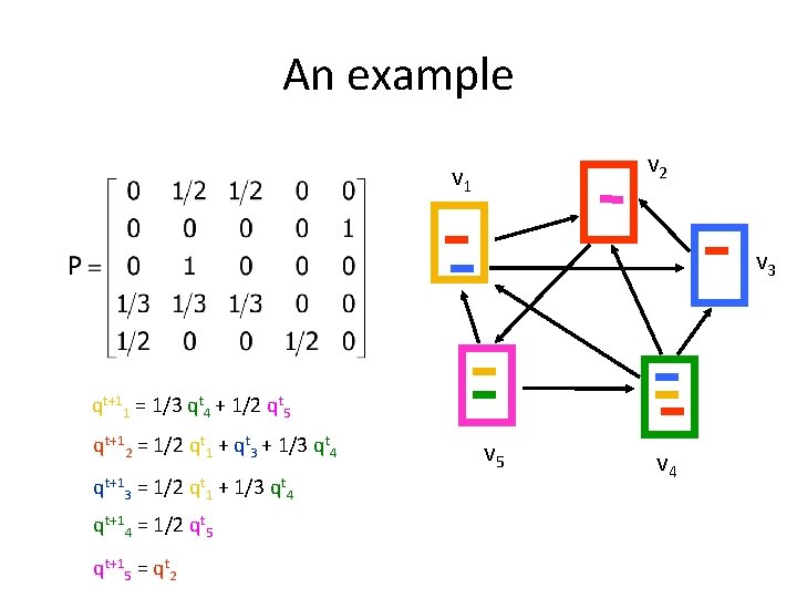
An example v 2 v 1 v 3 v 5 v 4

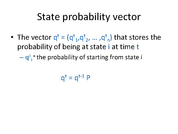
State probability vector • The vector qt = (qt 1, qt 2, … , qtn) that stores the probability of being at state i at time t – q 0 i = the probability of starting from state i qt = qt-1 P

An example v 2 v 1 v 3 qt+11 = 1/3 qt 4 + 1/2 qt 5 qt+12 = 1/2 qt 1 + qt 3 + 1/3 qt 4 qt+13 = 1/2 qt 1 + 1/3 qt 4 qt+14 = 1/2 qt 5 qt+15 = qt 2 v 5 v 4

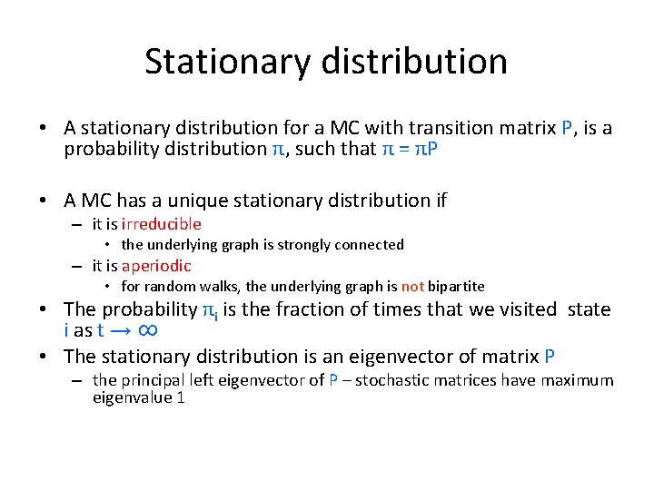
Stationary distribution • A stationary distribution for a MC with transition matrix P, is a probability distribution π, such that π = πP • A MC has a unique stationary distribution if – it is irreducible • the underlying graph is strongly connected – it is aperiodic • for random walks, the underlying graph is not bipartite • The probability πi is the fraction of times that we visited state i as t → ∞ • The stationary distribution is an eigenvector of matrix P – the principal left eigenvector of P – stochastic matrices have maximum eigenvalue 1

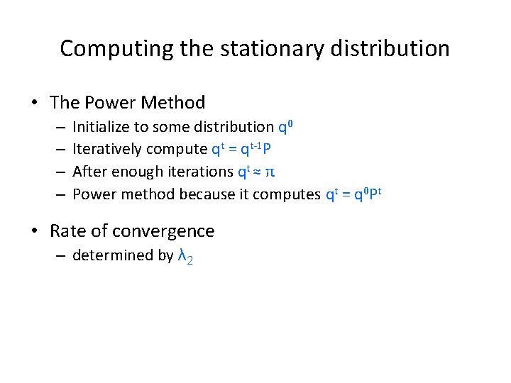
Computing the stationary distribution • The Power Method – – Initialize to some distribution q 0 Iteratively compute qt = qt-1 P After enough iterations qt ≈ π Power method because it computes qt = q 0 Pt • Rate of convergence – determined by λ 2

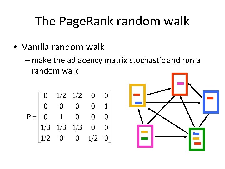
The Page. Rank random walk • Vanilla random walk – make the adjacency matrix stochastic and run a random walk

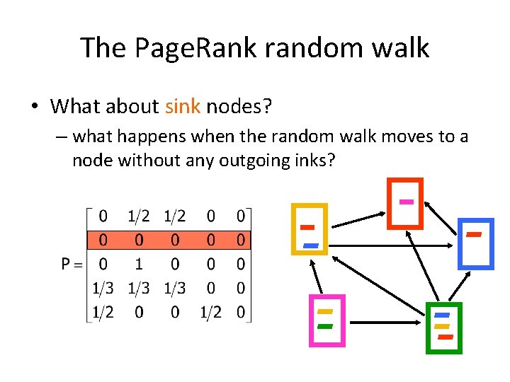
The Page. Rank random walk • What about sink nodes? – what happens when the random walk moves to a node without any outgoing inks?

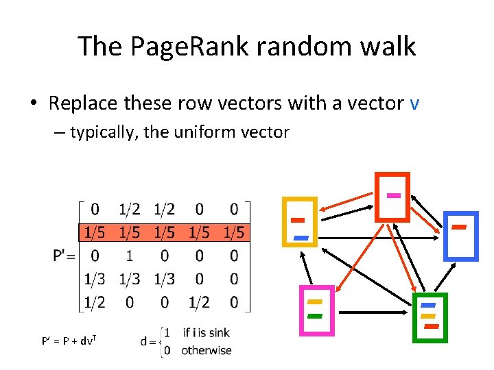
The Page. Rank random walk • Replace these row vectors with a vector v – typically, the uniform vector P’ = P + dv. T

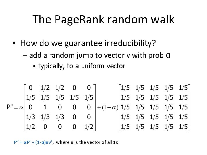
The Page. Rank random walk • How do we guarantee irreducibility? – add a random jump to vector v with prob α • typically, to a uniform vector P’’ = αP’ + (1 -α)uv. T, where u is the vector of all 1 s

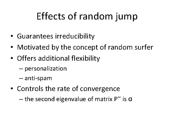
Effects of random jump • Guarantees irreducibility • Motivated by the concept of random surfer • Offers additional flexibility – personalization – anti-spam • Controls the rate of convergence – the second eigenvalue of matrix P’’ is α

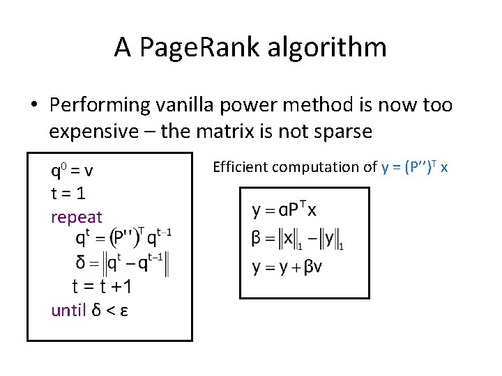
A Page. Rank algorithm • Performing vanilla power method is now too expensive – the matrix is not sparse q 0 = v t=1 repeat t = t +1 until δ < ε Efficient computation of y = (P’’)T x

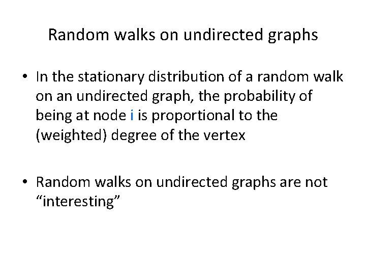
Random walks on undirected graphs • In the stationary distribution of a random walk on an undirected graph, the probability of being at node i is proportional to the (weighted) degree of the vertex • Random walks on undirected graphs are not “interesting”

Research on Page. Rank • Specialized Page. Rank – personalization [BP 98] • instead of picking a node uniformly at random favor specific nodes that are related to the user – topic sensitive Page. Rank [H 02] • compute many Page. Rank vectors, one for each topic • estimate relevance of query with each topic • produce final Page. Rank as a weighted combination • Updating Page. Rank [Chien et al 2002] • Fast computation of Page. Rank – numerical analysis tricks – node aggregation techniques – dealing with the “Web frontier”

Topic-sensitive pagerank • HITS-based scores are very inefficient to compute • Page. Rank scores are independent of the queries • Can we bias Page. Rank rankings to take into account query keywords? Topic-sensitive Page. Rank

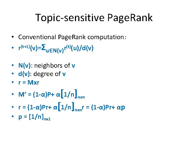
Topic-sensitive Page. Rank • Conventional Page. Rank computation: • r(t+1)(v)=ΣuЄN(v)r(t)(u)/d(v) • N(v): neighbors of v • d(v): degree of v • r = Mxr • M’ = (1 -α)P+ α[1/n]nxn • r = (1 -α)Pr+ α[1/n]nxnr = (1 -α)Pr+ αp • p = [1/n]nx 1

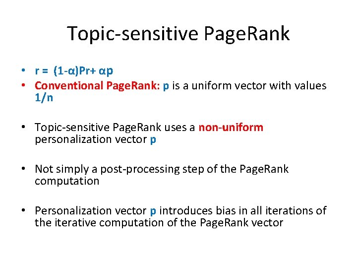
Topic-sensitive Page. Rank • r = (1 -α)Pr+ αp • Conventional Page. Rank: p is a uniform vector with values 1/n • Topic-sensitive Page. Rank uses a non-uniform personalization vector p • Not simply a post-processing step of the Page. Rank computation • Personalization vector p introduces bias in all iterations of the iterative computation of the Page. Rank vector

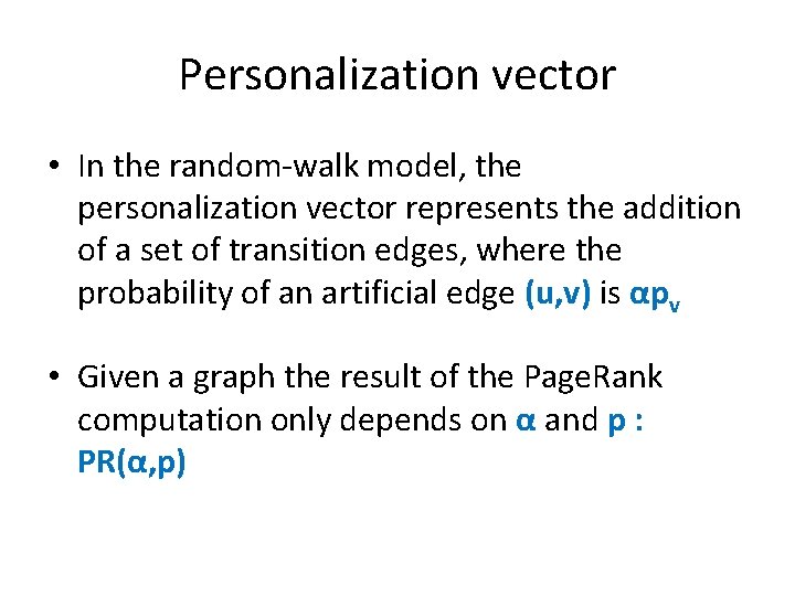
Personalization vector • In the random-walk model, the personalization vector represents the addition of a set of transition edges, where the probability of an artificial edge (u, v) is αpv • Given a graph the result of the Page. Rank computation only depends on α and p : PR(α, p)

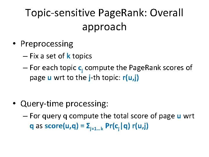
Topic-sensitive Page. Rank: Overall approach • Preprocessing – Fix a set of k topics – For each topic cj compute the Page. Rank scores of page u wrt to the j-th topic: r(u, j) • Query-time processing: – For query q compute the total score of page u wrt q as score(u, q) = Σj=1…k Pr(cj|q) r(u, j)

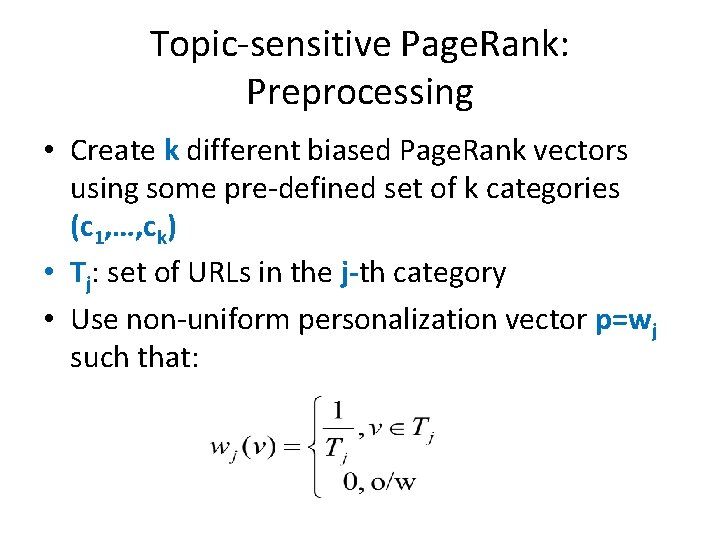
Topic-sensitive Page. Rank: Preprocessing • Create k different biased Page. Rank vectors using some pre-defined set of k categories (c 1, …, ck) • Tj: set of URLs in the j-th category • Use non-uniform personalization vector p=wj such that:

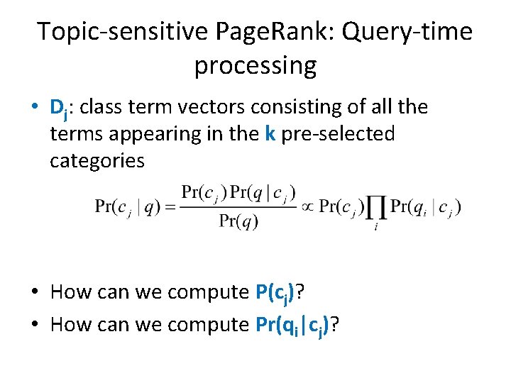
Topic-sensitive Page. Rank: Query-time processing • Dj: class term vectors consisting of all the terms appearing in the k pre-selected categories • How can we compute P(cj)? • How can we compute Pr(qi|cj)?

• Comparing results of Link Analysis Ranking algorithms • Comparing and aggregating rankings

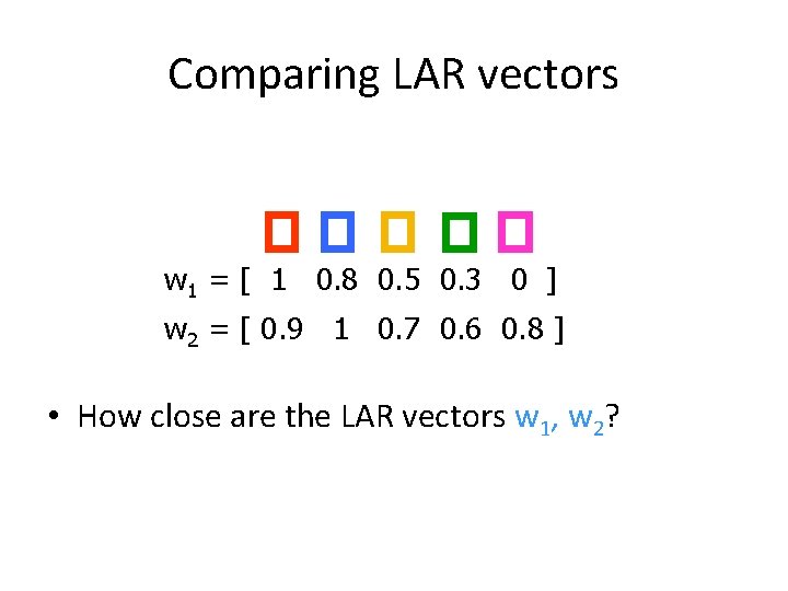
Comparing LAR vectors w 1 = [ 1 0. 8 0. 5 0. 3 0 ] w 2 = [ 0. 9 1 0. 7 0. 6 0. 8 ] • How close are the LAR vectors w 1, w 2?

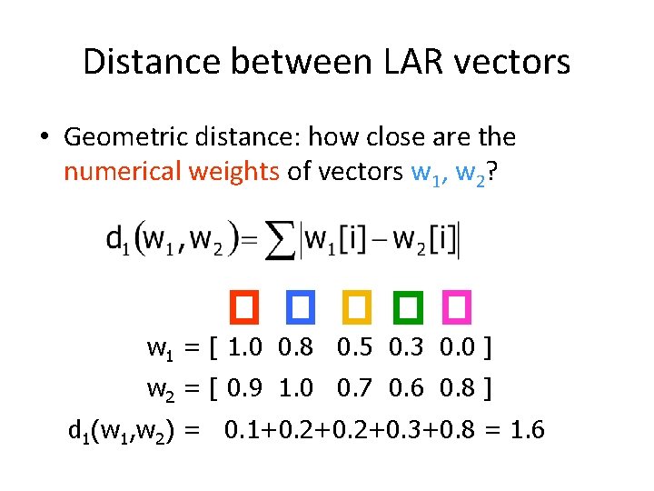
Distance between LAR vectors • Geometric distance: how close are the numerical weights of vectors w 1, w 2? w 1 = [ 1. 0 0. 8 0. 5 0. 3 0. 0 ] w 2 = [ 0. 9 1. 0 0. 7 0. 6 0. 8 ] d 1(w 1, w 2) = 0. 1+0. 2+0. 3+0. 8 = 1. 6

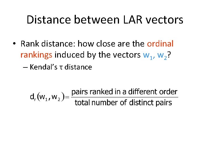
Distance between LAR vectors • Rank distance: how close are the ordinal rankings induced by the vectors w 1, w 2? – Kendal’s τ distance