Statistical Genomics Lecture 10 GWAS by Correlation Zhiwu

Statistical Genomics Lecture 10: GWAS by Correlation Zhiwu Zhang Washington State University

Outline • Correlation and t distribution • GWAS by correlation • Power and false positives • Observed null distribution • True positives • False positives • Type I error • Cut off of P values

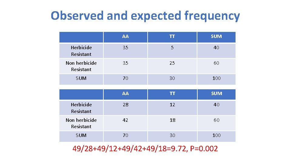
Observed and expected frequency AA TT SUM Herbicide Resistant 35 5 40 Non herbicide Resistant 35 25 60 SUM 70 30 100 AA TT SUM Herbicide Resistant 28 12 40 Non herbicide Resistant 42 18 60 SUM 70 30 100 49/28+49/12+49/42+49/18=9. 72, P=0. 002

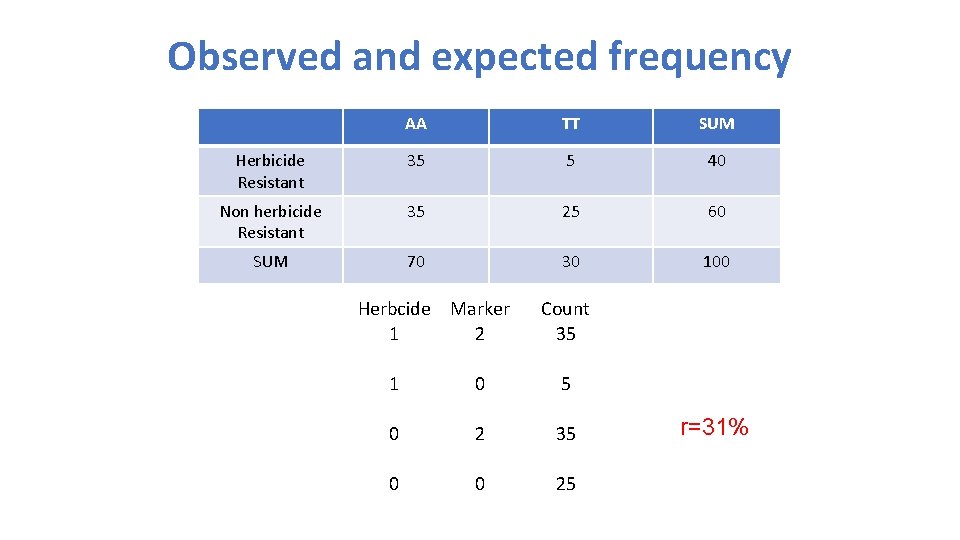
Observed and expected frequency AA TT SUM Herbicide Resistant 35 5 40 Non herbicide Resistant 35 25 60 SUM 70 30 100 Herbcide Marker 1 2 Count 35 1 0 5 0 2 35 0 0 25 r=31%

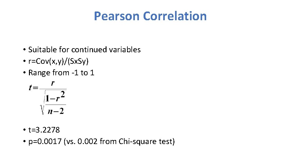
Pearson Correlation • Suitable for continued variables • r=Cov(x, y)/(Sx. Sy) • Range from -1 to 1 • t=3. 2278 • p=0. 0017 (vs. 0. 002 from Chi-square test)

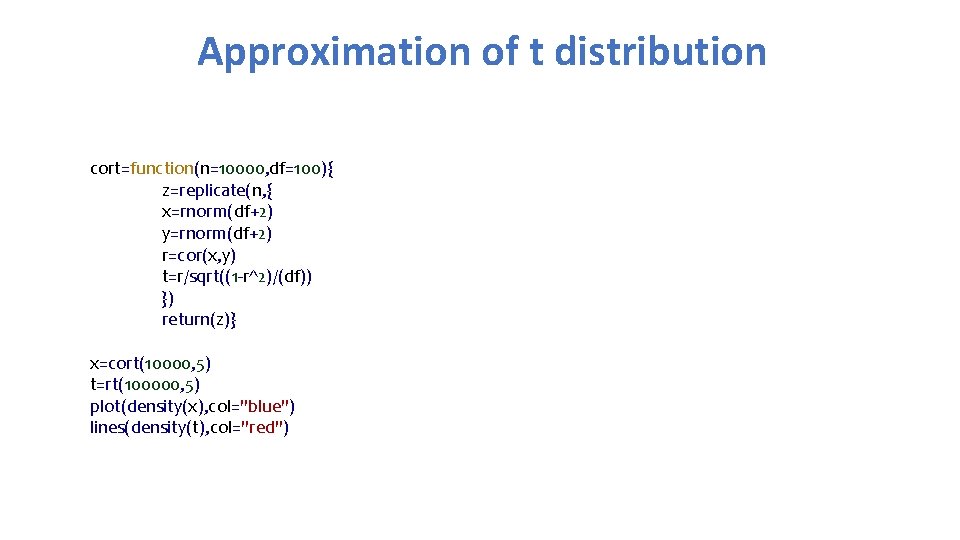
Approximation of t distribution cort=function(n=10000, df=100){ z=replicate(n, { x=rnorm(df+2) y=rnorm(df+2) r=cor(x, y) t=r/sqrt((1 -r^2)/(df)) }) return(z)} x=cort(10000, 5) t=rt(100000, 5) plot(density(x), col="blue") lines(density(t), col="red")

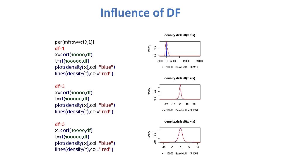
Influence of DF par(mfrow=c(3, 1)) df=1 x=cort(10000, df) t=rt(100000, df) plot(density(x), col="blue") lines(density(t), col="red") df=3 x=cort(10000, df) t=rt(100000, df) plot(density(x), col="blue") lines(density(t), col="red") df=5 x=cort(10000, df) t=rt(100000, df) plot(density(x), col="blue") lines(density(t), col="red")

Can we use correlation to map genes? • Try it • Sample ten SNPs as QTNs (mutations of genes) • Assign gene effects and make total genetic effects • Add residuals to make phenotypes with 75% heritability • Test all the SNPs and see how many can be found among the top ten associations.

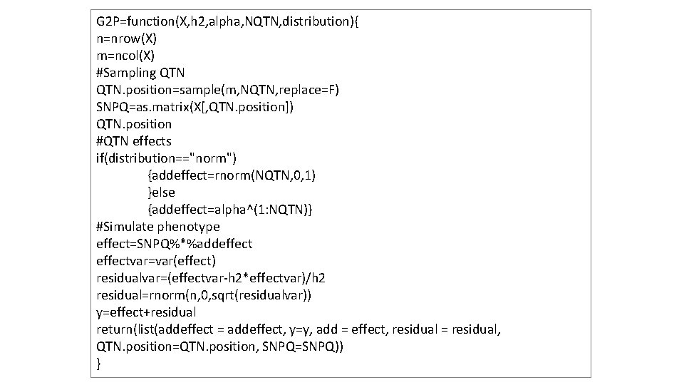
G 2 P=function(X, h 2, alpha, NQTN, distribution){ n=nrow(X) m=ncol(X) #Sampling QTN. position=sample(m, NQTN, replace=F) SNPQ=as. matrix(X[, QTN. position]) QTN. position #QTN effects if(distribution=="norm") {addeffect=rnorm(NQTN, 0, 1) }else {addeffect=alpha^(1: NQTN)} #Simulate phenotype effect=SNPQ%*%addeffectvar=var(effect) residualvar=(effectvar-h 2*effectvar)/h 2 residual=rnorm(n, 0, sqrt(residualvar)) y=effect+residual return(list(addeffect = addeffect, y=y, add = effect, residual = residual, QTN. position=QTN. position, SNPQ=SNPQ)) }

Read data and source code in R my. GD=read. table(file="http: //zzlab. net/GAPIT/data/mdp_numeric. txt", head=T) my. GM=read. table(file="http: //zzlab. net/GAPIT/data/mdp_SNP_information. txt", head=T) setwd("~/Dropbox/Current/ZZLab/WSUCourse/CROPS 545/Demo") source("G 2 P. R")

Let us have more fun! • Have the ten genes on chromosome 15 only, nothing on 6 to 10. • Any associations on chromosome 6 -10 should be false positives X=my. GD[, -1] index 1 to 5=my. GM[, 2]<6 X 1 to 5 = X[, index 1 to 5]

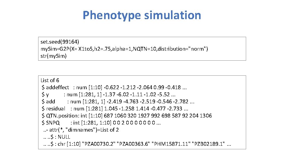
Phenotype simulation set. seed(99164) my. Sim=G 2 P(X= X 1 to 5, h 2=. 75, alpha=1, NQTN=10, distribution="norm") str(my. Sim) List of 6 $ addeffect : num [1: 10] -0. 622 -1. 212 -2. 064 0. 99 -0. 418. . . $y : num [1: 281, 1] -1. 37 -6. 02 -1. 11 -1. 02 -5. 52. . . $ add : num [1: 281, 1] -2. 419 -4. 763 -2. 519 -0. 546 -2. 782. . . $ residual : num [1: 281] 1. 045 -1. 258 1. 414 -0. 477 -2. 733. . . $ QTN. position: int [1: 10] 687 1060 320 1927 992 698 587 92 204 1306 $ SNPQ : int [1: 281, 1: 10] 0 0 2 0 0 0 0. . . - attr(*, "dimnames")=List of 2. . $ : NULL. . $ : chr [1: 10] "PZA 00730. 2" "PZA 00363. 6" "PHM 15871. 11" "PZB 02189. 1". . .

QTN positions plot(my. GM[, c(2, 3)]) lines(my. GM[my. Sim$QTN. position, c(2, 3)], type="p", col="red") points(my. GM[my. Sim$QTN. position, c(2, 3)], type="p", col="blue", cex = 5)

Association test by correlation r=cor(my. Sim$y, X) n=nrow(X) t=r/sqrt((1 -r^2)/(n-2)) p=2*(1 -pt(abs(t), n-2))

Manhattan plots color. vector <- rep(c("deepskyblue", "orange", "forestgreen", "indianred 3"), 10) m=ncol(X) plot(t(-log 10(p))~seq(1: m), col=color. vector[my. GM[, 2]]) abline(v=my. Sim$QTN. position, lty = 2, lwd=1. 5, col = "black")

Two additional findings sort(p)[1: 5] zeros=p==0 p[zeros]=1 e-10 plot(t(-log 10(p))~seq(1: m), col=color. vector[my. GM[, 2]]) abline(v=my. Sim$QTN. position, lty = 2, lwd=1. 5, col = "black")

GWAS by correlation GWASby. Cor=function(X, y){ n=nrow(X) r=cor(y, X) n=nrow(X) t=r/sqrt((1 -r^2)/(n-2)) p=2*(1 -pt(abs(t), n-2)) zeros=p==0 p[zeros]=1 e-10 return(p)}

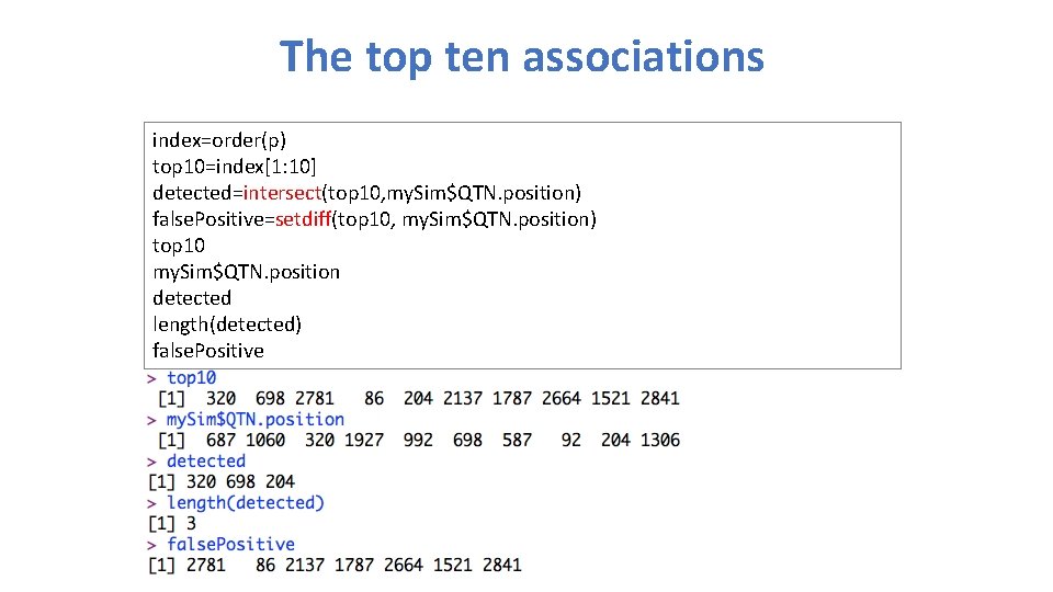
The top ten associations index=order(p) top 10=index[1: 10] detected=intersect(top 10, my. Sim$QTN. position) false. Positive=setdiff(top 10, my. Sim$QTN. position) top 10 my. Sim$QTN. position detected length(detected) false. Positive

The top ten associations plot(t(-log 10(p))~seq(1: m), col=color. vector[my. GM[, 2]]) abline(v=my. Sim$QTN. position, lty = 2, lwd=2, col = "black") abline(v= false. Positive, lty = 2, lwd=2, col = "red")

Null distribution of P values hist(p[!index 1 to 5])

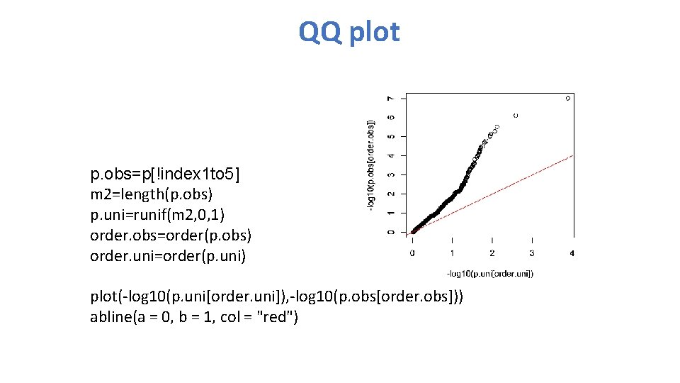
QQ plot p. obs=p[!index 1 to 5] m 2=length(p. obs) p. uni=runif(m 2, 0, 1) order. obs=order(p. obs) order. uni=order(p. uni) plot(-log 10(p. uni[order. uni]), -log 10(p. obs[order. obs])) abline(a = 0, b = 1, col = "red")

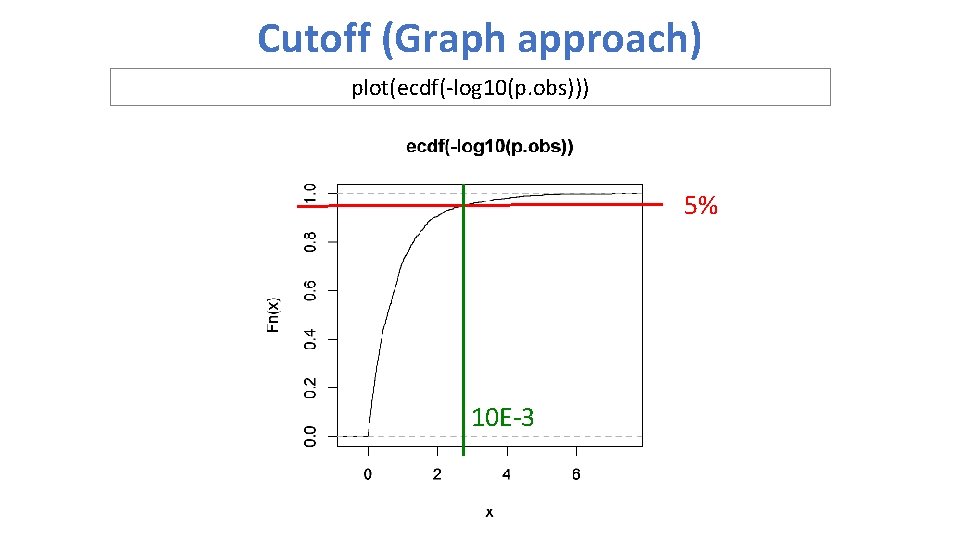
Cutoff (Graph approach) plot(ecdf(-log 10(p. obs))) 5% 10 E-3

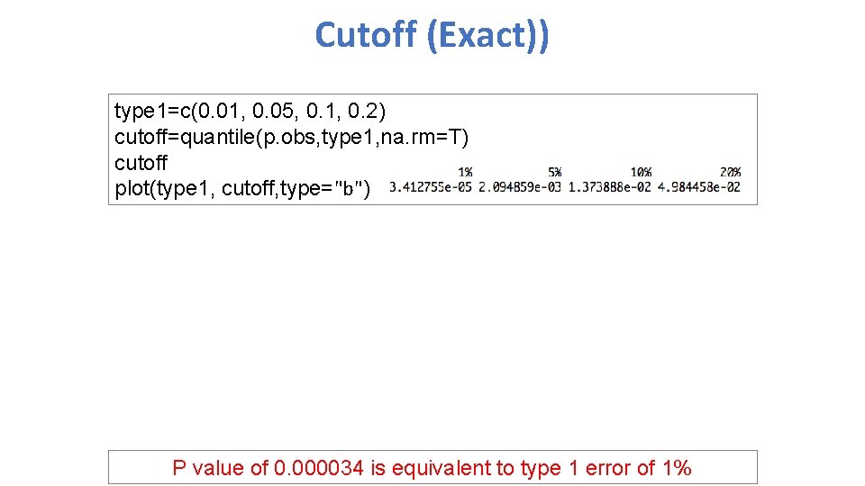
Cutoff (Exact)) type 1=c(0. 01, 0. 05, 0. 1, 0. 2) cutoff=quantile(p. obs, type 1, na. rm=T) cutoff plot(type 1, cutoff, type="b") P value of 0. 000034 is equivalent to type 1 error of 1%

Highlight • Correlation and t distribution • GWAS by correlation • Power and false positives • Observed null distribution • True positives • False positives • Type I error • Cut off of P values