Microsoft Excel Expert 2016 Lesson 1 Managing and

Microsoft Excel Expert 2016 Lesson 1 Managing and Protecting Workbooks © 2016, John Wiley & Sons, Inc. Microsoft Official Academic Course, Microsoft Excel Expert 2016 1

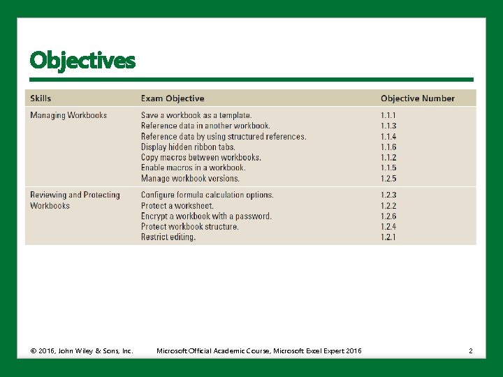
Objectives © 2016, John Wiley & Sons, Inc. Microsoft Official Academic Course, Microsoft Excel Expert 2016 2

Managing Workbooks • While using Excel, you will often need to perform workbook management tasks, for example: • You can modify an Excel template to suit your needs and save it as a custom template. • You may need to refer to cells in another worksheet in the same workbook or to another workbook entirely. • You can use structured references in tables, which use table names and column headings in formulas rather than cell references. This makes it easier for you and others to interpret workbook formulas. • You can easily display ribbon tabs that are hidden by default using the Excel Options dialog box. • You can copy macros between workbooks. • You can manage different versions of the same workbook. © 2016, John Wiley & Sons, Inc. Microsoft Official Academic Course, Microsoft Excel Expert 2016 3

Creating Custom Templates • Every time you open Excel, you see a listing of available templates (unless you change the default setting). • You can create your own custom templates. • You can create an Excel template completely from scratch. • You can also modify a preinstalled template and save it as your own custom template. © 2016, John Wiley & Sons, Inc. Microsoft Official Academic Course, Microsoft Excel Expert 2016 4

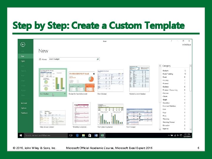
Step by Step: Create a Custom Template • LAUNCH Excel 2016 if it is not already open. 1. If you just opened Excel, you’re looking at the list of featured templates. If you do not see the list of featured templates, click the File tab and then click New. 2. Click in the Search for online templates box, type Event budget, and then press Enter. 3. The Event budget template now displays at the beginning of the templates listing (see the figure on the next slide). Select the Event budget template. Click the Create button in the preview window. © 2016, John Wiley & Sons, Inc. Microsoft Official Academic Course, Microsoft Excel Expert 2016 5

Step by Step: Create a Custom Template © 2016, John Wiley & Sons, Inc. Microsoft Official Academic Course, Microsoft Excel Expert 2016 6

Step by Step: Create a Custom Template 4. 5. 6. 7. 8. 9. Select cell B 2 on the DASHBOARD worksheet and edit the value to read: Budget for Training Seminar in [City, State] Scroll down the worksheet as necessary and then click the pie chart with the title Actual. Click the Chart Tools Design tab and then use the Chart Styles gallery to change the pie chart’s style to Style 1. Click the column chart with the title Total Profit and change the column chart’s style to Style 4. Select the INCOME worksheet. Delete rows 13: 26. Fix the formulas in cells F 5 and G 5 by deleting the #REF! arguments (and the comma that follows the argument) in each formula. Select the DASHBOARD worksheet. Click the Page Layout tab. Click the Themes button and then select the Dividend theme. © 2016, John Wiley & Sons, Inc. Microsoft Official Academic Course, Microsoft Excel Expert 2016 7

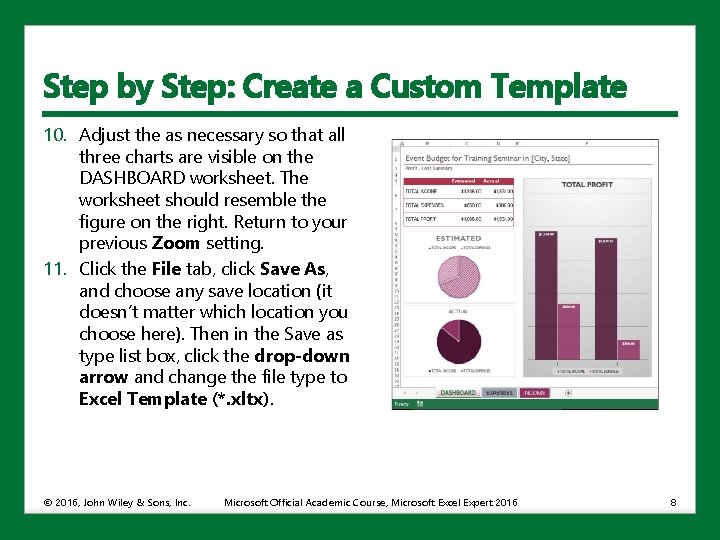
Step by Step: Create a Custom Template 10. Adjust the as necessary so that all three charts are visible on the DASHBOARD worksheet. The worksheet should resemble the figure on the right. Return to your previous Zoom setting. 11. Click the File tab, click Save As, and choose any save location (it doesn’t matter which location you choose here). Then in the Save as type list box, click the drop-down arrow and change the file type to Excel Template (*. xltx). © 2016, John Wiley & Sons, Inc. Microsoft Official Academic Course, Microsoft Excel Expert 2016 8

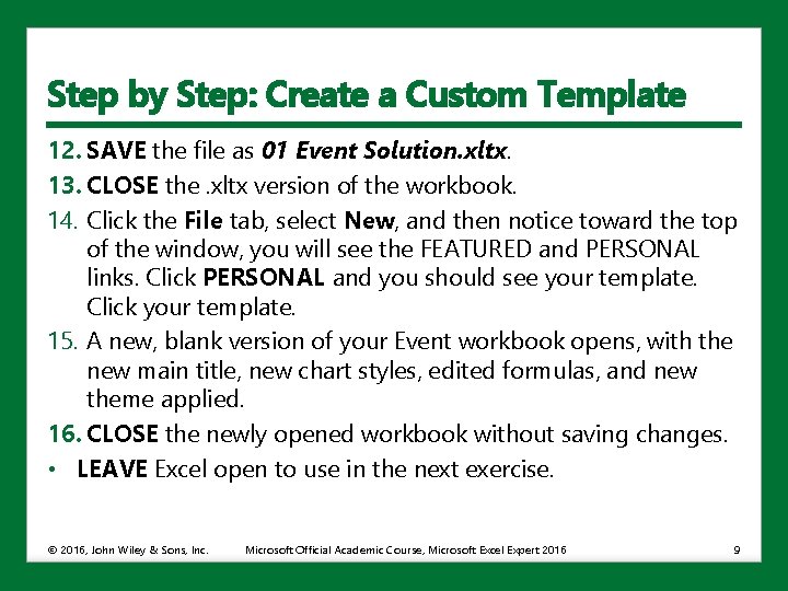
Step by Step: Create a Custom Template 12. SAVE the file as 01 Event Solution. xltx. 13. CLOSE the. xltx version of the workbook. 14. Click the File tab, select New, and then notice toward the top of the window, you will see the FEATURED and PERSONAL links. Click PERSONAL and you should see your template. Click your template. 15. A new, blank version of your Event workbook opens, with the new main title, new chart styles, edited formulas, and new theme applied. 16. CLOSE the newly opened workbook without saving changes. • LEAVE Excel open to use in the next exercise. © 2016, John Wiley & Sons, Inc. Microsoft Official Academic Course, Microsoft Excel Expert 2016 9

Referencing Data in Another Worksheet • When entering formulas in a worksheet, you might need to refer to a cell or range in another worksheet within the same workbook. • You could use this strategy, for example, to create a summary of data in one worksheet based on data in another worksheet. • The basic principles for building these formulas are similar to those for building formulas referencing data within a worksheet. © 2016, John Wiley & Sons, Inc. Microsoft Official Academic Course, Microsoft Excel Expert 2016 10

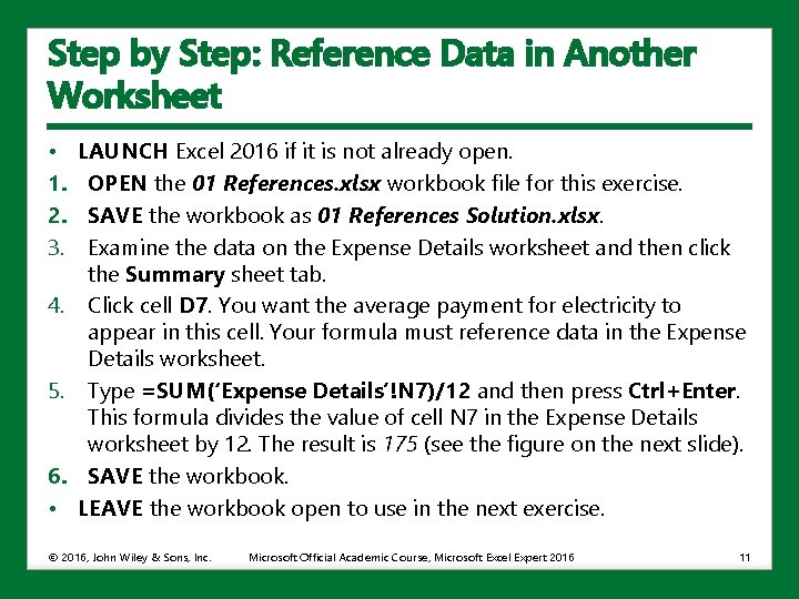
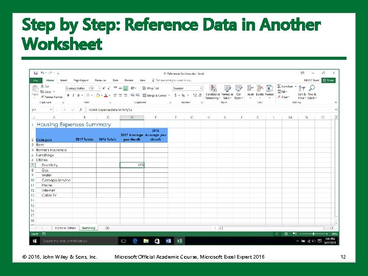
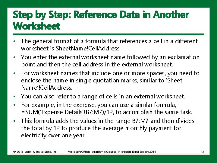
Step by Step: Reference Data in Another Worksheet • 1. 2. 3. 4. 5. 6. • LAUNCH Excel 2016 if it is not already open. OPEN the 01 References. xlsx workbook file for this exercise. SAVE the workbook as 01 References Solution. xlsx. Examine the data on the Expense Details worksheet and then click the Summary sheet tab. Click cell D 7. You want the average payment for electricity to appear in this cell. Your formula must reference data in the Expense Details worksheet. Type =SUM(‘Expense Details’!N 7)/12 and then press Ctrl+Enter. This formula divides the value of cell N 7 in the Expense Details worksheet by 12. The result is 175 (see the figure on the next slide). SAVE the workbook. LEAVE the workbook open to use in the next exercise. © 2016, John Wiley & Sons, Inc. Microsoft Official Academic Course, Microsoft Excel Expert 2016 11

Step by Step: Reference Data in Another Worksheet © 2016, John Wiley & Sons, Inc. Microsoft Official Academic Course, Microsoft Excel Expert 2016 12

Step by Step: Reference Data in Another Worksheet • The general format of a formula that references a cell in a different worksheet is Sheet. Name!Cell. Address. • You enter the external worksheet name followed by an exclamation point and then the cell address in the external worksheet. • For worksheet names that include one or more spaces, you need to enclose the name in single quotation marks, similar to ‘Sheet Name’!Cell. Address. • You can also refer to a range of cells in an external worksheet. • For example, in the exercise, you can use a similar formula, =SUM(‘Expense Details’!B 7: M 7)/12, to accomplish the same task. • This formula adds the values in the range B 7: M 7 and then divides the total by 12 to produce the average monthly payment for electricity over one year. © 2016, John Wiley & Sons, Inc. Microsoft Official Academic Course, Microsoft Excel Expert 2016 13

Referencing Data in Another Workbook • The procedure for referencing data in another workbook is nearly the same as referencing data in another worksheet in the same workbook. • The difference is that, when referring to cells in another workbook, you must enclose the other workbook name in square brackets ([ ]) and both workbooks must be open. © 2016, John Wiley & Sons, Inc. Microsoft Official Academic Course, Microsoft Excel Expert 2016 14

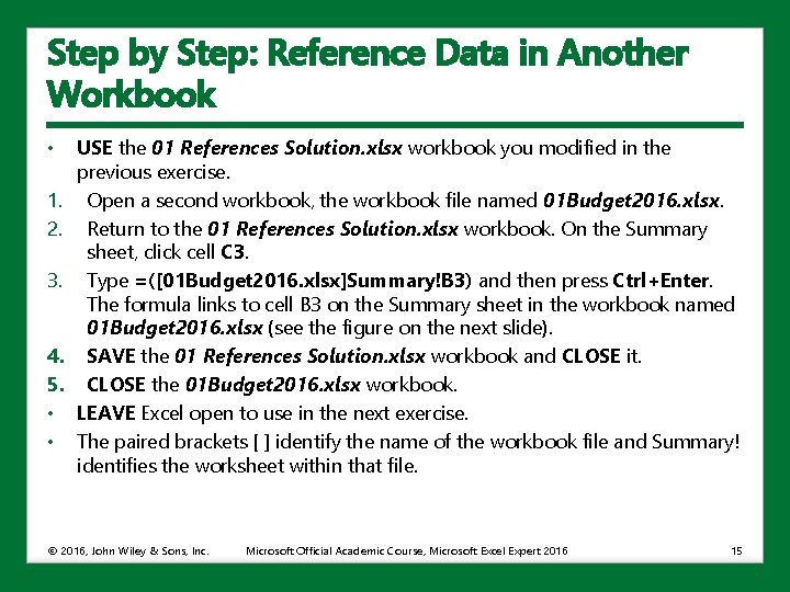
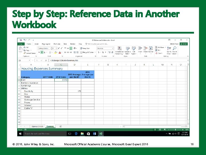
Step by Step: Reference Data in Another Workbook • 1. 2. 3. 4. 5. • • USE the 01 References Solution. xlsx workbook you modified in the previous exercise. Open a second workbook, the workbook file named 01 Budget 2016. xlsx. Return to the 01 References Solution. xlsx workbook. On the Summary sheet, click cell C 3. Type =([01 Budget 2016. xlsx]Summary!B 3) and then press Ctrl+Enter. The formula links to cell B 3 on the Summary sheet in the workbook named 01 Budget 2016. xlsx (see the figure on the next slide). SAVE the 01 References Solution. xlsx workbook and CLOSE it. CLOSE the 01 Budget 2016. xlsx workbook. LEAVE Excel open to use in the next exercise. The paired brackets [ ] identify the name of the workbook file and Summary! identifies the worksheet within that file. © 2016, John Wiley & Sons, Inc. Microsoft Official Academic Course, Microsoft Excel Expert 2016 15

Step by Step: Reference Data in Another Workbook © 2016, John Wiley & Sons, Inc. Microsoft Official Academic Course, Microsoft Excel Expert 2016 16

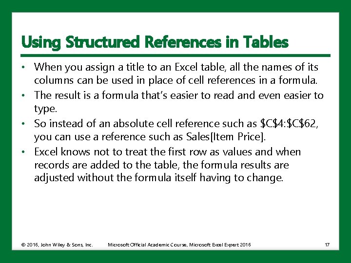
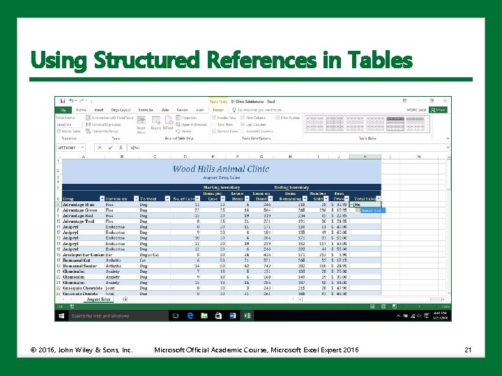
Using Structured References in Tables • When you assign a title to an Excel table, all the names of its columns can be used in place of cell references in a formula. • The result is a formula that’s easier to read and even easier to type. • So instead of an absolute cell reference such as $C$4: $C$62, you can use a reference such as Sales[Item Price]. • Excel knows not to treat the first row as values and when records are added to the table, the formula results are adjusted without the formula itself having to change. © 2016, John Wiley & Sons, Inc. Microsoft Official Academic Course, Microsoft Excel Expert 2016 17

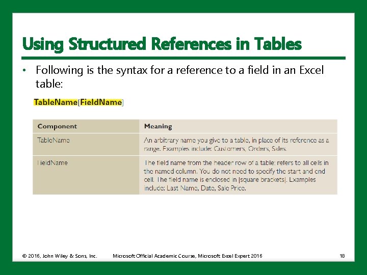
Using Structured References in Tables • Following is the syntax for a reference to a field in an Excel table: © 2016, John Wiley & Sons, Inc. Microsoft Official Academic Course, Microsoft Excel Expert 2016 18

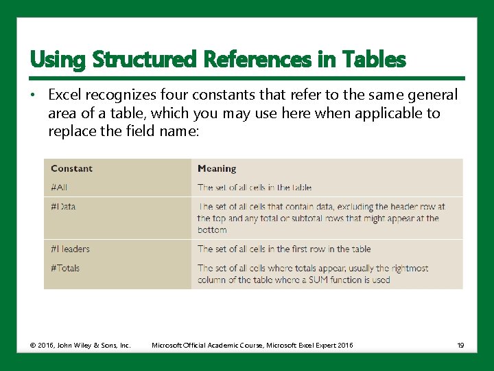
Using Structured References in Tables • Excel recognizes four constants that refer to the same general area of a table, which you may use here when applicable to replace the field name: © 2016, John Wiley & Sons, Inc. Microsoft Official Academic Course, Microsoft Excel Expert 2016 19

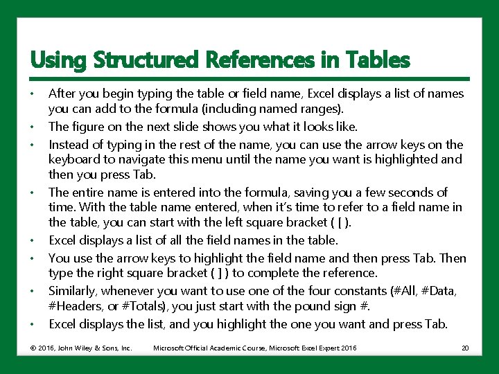
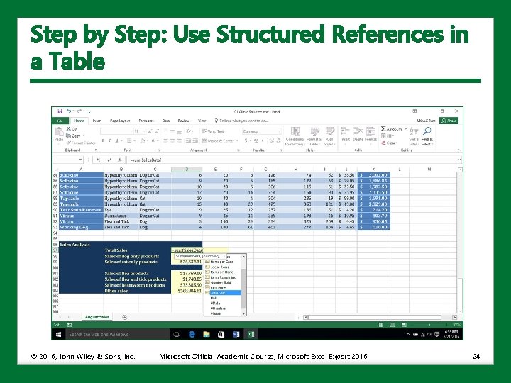
Using Structured References in Tables • • After you begin typing the table or field name, Excel displays a list of names you can add to the formula (including named ranges). The figure on the next slide shows you what it looks like. Instead of typing in the rest of the name, you can use the arrow keys on the keyboard to navigate this menu until the name you want is highlighted and then you press Tab. The entire name is entered into the formula, saving you a few seconds of time. With the table name entered, when it’s time to refer to a field name in the table, you can start with the left square bracket ( [ ). Excel displays a list of all the field names in the table. You use the arrow keys to highlight the field name and then press Tab. Then type the right square bracket ( ] ) to complete the reference. Similarly, whenever you want to use one of the four constants (#All, #Data, #Headers, or #Totals), you just start with the pound sign #. Excel displays the list, and you highlight the one you want and press Tab. © 2016, John Wiley & Sons, Inc. Microsoft Official Academic Course, Microsoft Excel Expert 2016 20

Using Structured References in Tables © 2016, John Wiley & Sons, Inc. Microsoft Official Academic Course, Microsoft Excel Expert 2016 21

Step by Step: Use Structured References in a Table • 1. 2. 3. 4. 5. 6. 7. LAUNCH Excel 2016 if it is not already open. OPEN the 01 Clinic. xlsx workbook file for this exercise. SAVE the workbook as 01 Clinic Solution. xlsx. In the August Sales worksheet, click anywhere inside the table that begins in row 6. Click the Design tab, and then in the Properties group, click the text box under Table Name. Type Sales. Data (all one word) and then press Enter. You have given a name to the table. Now you can replace formulas at the bottom of the August Sales worksheet with formulas that are easier to read, yet yield the same results. Select cell D 97 (Total Sales). Type =sum(Sa © 2016, John Wiley & Sons, Inc. Microsoft Official Academic Course, Microsoft Excel Expert 2016 22

Step by Step: Use Structured References in a Table 8. When Sales. Data appears in the list, press Tab. 9. Type [ (left square bracket). 10. Use the arrow keys to select Total Sales from the list (see the figure on the next slide) and then press Tab. 11. Type ] (right square bracket), followed by ) (right parenthesis) and then press Enter. If you enter the formula properly, the result should be identical to what was there before. 12. Replace the formula in cell D 98 with the following: 13. =SUMIF(Sales. Data[To treat], ”Dog”, Sales. Data[Total Sales]) 14. Replace the formula in cell D 99 with one based on the formula in D 98, but searching for Cat instead of Dog. 15. SAVE the workbook and CLOSE it. 16. LEAVE Excel open for the next exercise. © 2016, John Wiley & Sons, Inc. Microsoft Official Academic Course, Microsoft Excel Expert 2016 23

Step by Step: Use Structured References in a Table © 2016, John Wiley & Sons, Inc. Microsoft Official Academic Course, Microsoft Excel Expert 2016 24

Displaying Hidden Tabs on the Ribbon • Most of Excel’s ribbon tabs display on the ribbon by default, or appear automatically as contextual tabs when you perform certain tasks (such as working with tables or graphics). • However, you must manually display certain ribbon tabs, such as the Developer tab, when you need them. • You can use the Excel Options dialog box to display (or later remove) these hidden tabs. © 2016, John Wiley & Sons, Inc. Microsoft Official Academic Course, Microsoft Excel Expert 2016 25

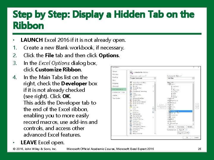
Step by Step: Display a Hidden Tab on the Ribbon • LAUNCH Excel 2016 if it is not already open. 1. Create a new Blank workbook, if necessary. 2. Click the File tab and then click Options. 3. In the Excel Options dialog box, click Customize Ribbon. 4. In the Main Tabs list on the right, check the Developer box if it is not already checked (see right). Click OK. This adds the Developer tab to the end of the Excel ribbon, enabling you to more easily record macros, use add-ins and controls, and access other advanced Excel features. • LEAVE Excel open. © 2016, John Wiley & Sons, Inc. Microsoft Official Academic Course, Microsoft Excel Expert 2016 26

Copying Macros between Workbooks • Another aspect of workbook management is transferring macros from one workbook to another. • You might have a workbook where several helpful macros have been written and you would like to make use of those tools in your own workbook. © 2016, John Wiley & Sons, Inc. Microsoft Official Academic Course, Microsoft Excel Expert 2016 27

Step by Step: Copy a Macro to Another Workbook • LAUNCH Excel 2016 if it is not already open. 1. OPEN the 01 Macros. xlsm workbook file for this exercise. If you see a yellow message bar, click the Enable Content button. 2. Once you have the workbook open, click each of the three buttons in succession, to observe the macro attached to each button execute. (After you click the first button, you will need to click OK in the resulting message box to continue. ) 3. Press Ctrl+N to create a new workbook. SAVE the workbook in Excel Macro -Enabled Workbook (*. xlsm) format as 01 Macros Solution. xlsm. 4. Ensure that you have the Developer tab displayed in the ribbon. (Refer to the previous section, “Displaying Hidden Tabs on the Ribbon, ” if necessary. ) Click the Developer tab and then in the Code group, click the Visual Basic button. This will open the Visual Basic Editor (VBE). Maximize the VBE window, if necessary. Then, maximize the Code window in the right pane, if necessary. © 2016, John Wiley & Sons, Inc. Microsoft Official Academic Course, Microsoft Excel Expert 2016 28

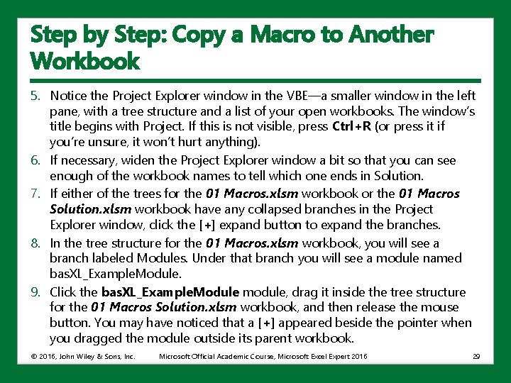
Step by Step: Copy a Macro to Another Workbook 5. Notice the Project Explorer window in the VBE—a smaller window in the left pane, with a tree structure and a list of your open workbooks. The window’s title begins with Project. If this is not visible, press Ctrl+R (or press it if you’re unsure, it won’t hurt anything). 6. If necessary, widen the Project Explorer window a bit so that you can see enough of the workbook names to tell which one ends in Solution. 7. If either of the trees for the 01 Macros. xlsm workbook or the 01 Macros Solution. xlsm workbook have any collapsed branches in the Project Explorer window, click the [+] expand button to expand the branches. 8. In the tree structure for the 01 Macros. xlsm workbook, you will see a branch labeled Modules. Under that branch you will see a module named bas. XL_Example. Module. 9. Click the bas. XL_Example. Module module, drag it inside the tree structure for the 01 Macros Solution. xlsm workbook, and then release the mouse button. You may have noticed that a [+] appeared beside the pointer when you dragged the module outside its parent workbook. © 2016, John Wiley & Sons, Inc. Microsoft Official Academic Course, Microsoft Excel Expert 2016 29

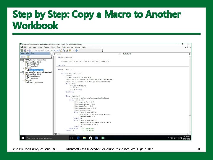
Step by Step: Copy a Macro to Another Workbook 10. The tree structure under the 01 Macros Solution. xlsm workbook will now have a Modules folder. Click the [+] expand button to expand the folder (see the figure on the next slide). 11. In the VBE window, click File and then click Close and Return to Microsoft Excel. Display the new 01 Macros Solution. xlsm workbook, if necessary. 12. On the Developer tab, in the Code group, click the Macros button. In the Macro dialog box, change the Macros in value to This Workbook. Then, in the list box, select the Hello. World macro and click the Run button. Click OK to close the resulting message box. 13. Repeat step 12 to run the Hello. Cells macro. 14. Repeat step 12 to run the Goodbye. Cells macro to clear the changes made in step 13. You just transferred three macros from one workbook to another. 15. SAVE the 01 Macros Solution. xlsm workbook and CLOSE it. Then, CLOSE the 01 Macros. xlsm workbook without saving changes. • CLOSE Excel. © 2016, John Wiley & Sons, Inc. Microsoft Official Academic Course, Microsoft Excel Expert 2016 30

Step by Step: Copy a Macro to Another Workbook © 2016, John Wiley & Sons, Inc. Microsoft Official Academic Course, Microsoft Excel Expert 2016 31

Managing Workbook Versions • Office 2016 includes an Auto. Recover feature that saves copies of your files at specified intervals. • The default setting is every 10 minutes; you can change this setting to another value. • Auto. Recover is useful: • If Excel (or another Office program) unexpectedly closes • If you accidentally close a file without saving changes • In the event of a power failure • If any of these events happen while you are working in Excel, you will see a Document Recovery pane with file recovery options the next time you open Excel. © 2016, John Wiley & Sons, Inc. Microsoft Official Academic Course, Microsoft Excel Expert 2016 32

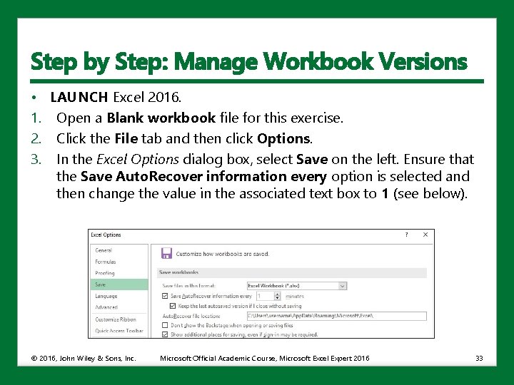
Step by Step: Manage Workbook Versions • LAUNCH Excel 2016. 1. Open a Blank workbook file for this exercise. 2. Click the File tab and then click Options. 3. In the Excel Options dialog box, select Save on the left. Ensure that the Save Auto. Recover information every option is selected and then change the value in the associated text box to 1 (see below). © 2016, John Wiley & Sons, Inc. Microsoft Official Academic Course, Microsoft Excel Expert 2016 33

Step by Step: Manage Workbook Versions 4. 5. 6. 7. 8. Select the Keep the last autosaved version if I close without saving check box, if it isn’t already selected. Click OK. Type your name (or any text) in cell A 1 and then press Enter. Wait at least one minute (so that Excel will autosave the file using the setting you changed in step 3). Then, right-click the Windows taskbar and select Task Manager from the shortcut menu. The Task Manager window displays. On the Processes tab, click Microsoft Excel in the Apps list. Click the End task button. Microsoft Excel closes. CLOSE the Task Manager window. OPEN Excel and click the Show Recovered Files option in the left pane. (If you don’t see this option, you probably didn’t wait long enough in step 6— select Blank workbook and repeat steps 5 -8. ) Excel opens a blank workbook and displays the Document Recovery task pane. © 2016, John Wiley & Sons, Inc. Microsoft Official Academic Course, Microsoft Excel Expert 2016 34

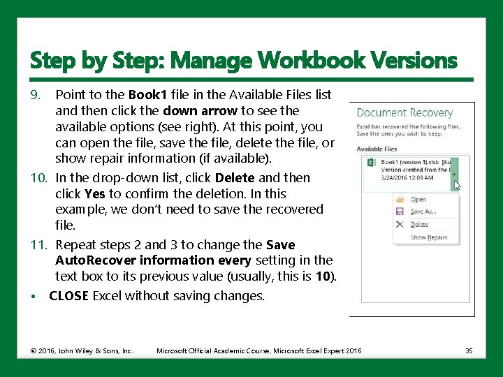
Step by Step: Manage Workbook Versions 9. Point to the Book 1 file in the Available Files list and then click the down arrow to see the available options (see right). At this point, you can open the file, save the file, delete the file, or show repair information (if available). 10. In the drop-down list, click Delete and then click Yes to confirm the deletion. In this example, we don’t need to save the recovered file. 11. Repeat steps 2 and 3 to change the Save Auto. Recover information every setting in the text box to its previous value (usually, this is 10). • CLOSE Excel without saving changes. © 2016, John Wiley & Sons, Inc. Microsoft Official Academic Course, Microsoft Excel Expert 2016 35

Step by Step: Manage Workbook Versions • Another way to access unsaved workbook files (if they are available) is by using the Info tab in Backstage view. 1. From the Info tab, click Manage Workbook and then select Recover Unsaved Workbooks. 2. Select a file you want to recover in the Open dialog box and then click Open. 3. Click the Save As button in the message bar and save the file if you want to keep it. 4. If you have one or more recent copies of unsaved files that you want to delete, from the Info tab in Backstage view, click Manage Workbook and then select Delete All Unsaved Workbooks. 5. Click Yes to confirm the deletion. © 2016, John Wiley & Sons, Inc. Microsoft Official Academic Course, Microsoft Excel Expert 2016 36

Reviewing and Protecting Workbooks • Excel provides calculation options that enable you to specify whether you want formula calculations to update automatically (the default setting) or manually. • You can also specify that data tables in a large workbook should be skipped but all other worksheet data should be updated automatically. • Then, you can update the data tables manually, as needed. • When sharing workbooks, you can protect an entire workbook by restricting who can open and/or use the workbook data and by requiring a password to view and/or save changes to the workbook. • You can also provide additional protection for certain worksheets or workbook elements with or without applying a password. © 2016, John Wiley & Sons, Inc. Microsoft Official Academic Course, Microsoft Excel Expert 2016 37

Setting Calculation Options • When working in Excel, you may occasionally work with a very large workbook with recalculation times that are becoming problematic. • Or you may find yourself in a situation where the solution to your problem requires iterative calculation (more commonly called a circular reference). • For this example, do not worry if Excel displays messages warning about the workbook containing circular references. © 2016, John Wiley & Sons, Inc. Microsoft Official Academic Course, Microsoft Excel Expert 2016 38

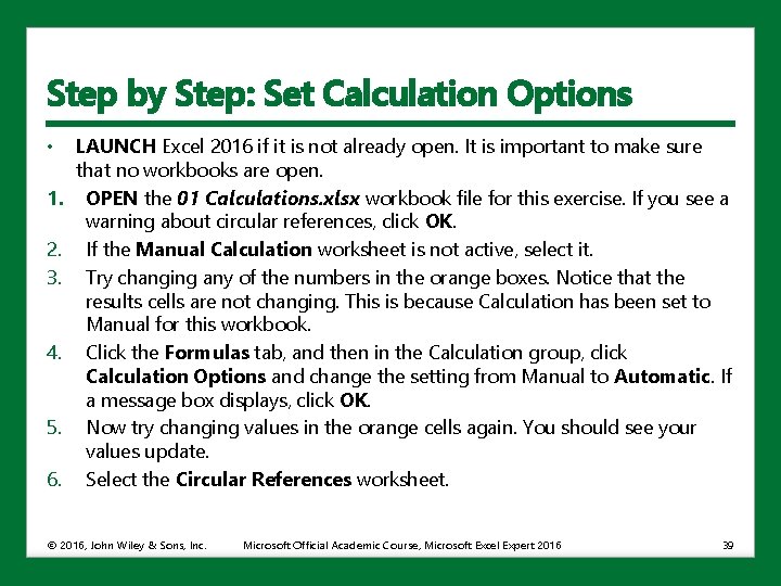
Step by Step: Set Calculation Options • 1. 2. 3. 4. 5. 6. LAUNCH Excel 2016 if it is not already open. It is important to make sure that no workbooks are open. OPEN the 01 Calculations. xlsx workbook file for this exercise. If you see a warning about circular references, click OK. If the Manual Calculation worksheet is not active, select it. Try changing any of the numbers in the orange boxes. Notice that the results cells are not changing. This is because Calculation has been set to Manual for this workbook. Click the Formulas tab, and then in the Calculation group, click Calculation Options and change the setting from Manual to Automatic. If a message box displays, click OK. Now try changing values in the orange cells again. You should see your values update. Select the Circular References worksheet. © 2016, John Wiley & Sons, Inc. Microsoft Official Academic Course, Microsoft Excel Expert 2016 39

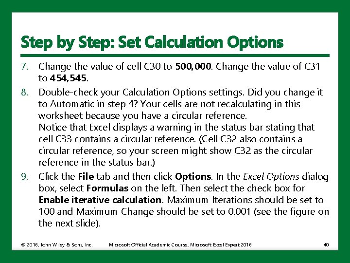
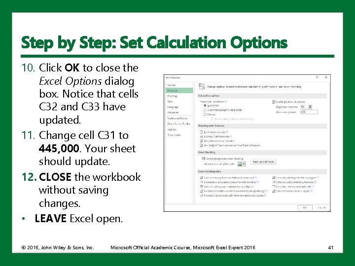
Step by Step: Set Calculation Options 7. 8. 9. Change the value of cell C 30 to 500, 000. Change the value of C 31 to 454, 545. Double-check your Calculation Options settings. Did you change it to Automatic in step 4? Your cells are not recalculating in this worksheet because you have a circular reference. Notice that Excel displays a warning in the status bar stating that cell C 33 contains a circular reference. (Cell C 32 also contains a circular reference, so your screen might show C 32 as the circular reference in the status bar. ) Click the File tab and then click Options. In the Excel Options dialog box, select Formulas on the left. Then select the check box for Enable iterative calculation. Maximum Iterations should be set to 100 and Maximum Change should be set to 0. 001 (see the figure on the next slide). © 2016, John Wiley & Sons, Inc. Microsoft Official Academic Course, Microsoft Excel Expert 2016 40

Step by Step: Set Calculation Options 10. Click OK to close the Excel Options dialog box. Notice that cells C 32 and C 33 have updated. 11. Change cell C 31 to 445, 000. Your sheet should update. 12. CLOSE the workbook without saving changes. • LEAVE Excel open. © 2016, John Wiley & Sons, Inc. Microsoft Official Academic Course, Microsoft Excel Expert 2016 41

Protecting a Worksheet • In a work environment, workbooks are frequently used by more than one employee. • When you create a worksheet that is accessed by multiple users, you often need to protect it so that a user does not accidentally or intentionally change, move, or delete important data. © 2016, John Wiley & Sons, Inc. Microsoft Official Academic Course, Microsoft Excel Expert 2016 42

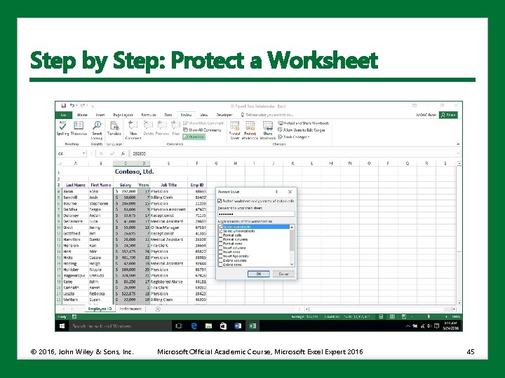
Step by Step: Protect a Worksheet • LAUNCH Excel 2016 if it is not already open. 1. OPEN the 01 Payroll Data. xlsx workbook from the data files for this lesson. 2. SAVE the workbook as 01 Payroll Data Solution. xlsx. 3. On the Employee ID worksheet, select the range F 4: F 33. 4. With F 4: F 33 selected, on the Home tab, in the Cells group, click Format and then select Format Cells. Click the Protection tab and verify that Locked is checked. This prevents employee ID numbers from being changed when the worksheet has been protected. Click OK. 5. Select cells C 4: D 33. On the Home tab, click Format. Notice that the Lock Cell command appears selected, meaning the cells are locked by default. Click Lock Cell to turn off the protection on these cells to allow these cells to change. 6. Click the Review tab, and in the Changes group, click Protect Sheet. © 2016, John Wiley & Sons, Inc. Microsoft Official Academic Course, Microsoft Excel Expert 2016 43

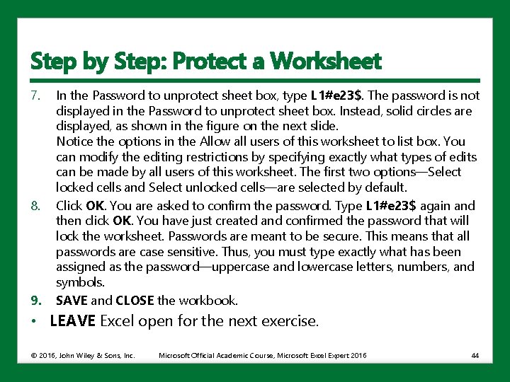
Step by Step: Protect a Worksheet 7. 8. 9. In the Password to unprotect sheet box, type L 1#e 23$. The password is not displayed in the Password to unprotect sheet box. Instead, solid circles are displayed, as shown in the figure on the next slide. Notice the options in the Allow all users of this worksheet to list box. You can modify the editing restrictions by specifying exactly what types of edits can be made by all users of this worksheet. The first two options—Select locked cells and Select unlocked cells—are selected by default. Click OK. You are asked to confirm the password. Type L 1#e 23$ again and then click OK. You have just created and confirmed the password that will lock the worksheet. Passwords are meant to be secure. This means that all passwords are case sensitive. Thus, you must type exactly what has been assigned as the password—uppercase and lowercase letters, numbers, and symbols. SAVE and CLOSE the workbook. • LEAVE Excel open for the next exercise. © 2016, John Wiley & Sons, Inc. Microsoft Official Academic Course, Microsoft Excel Expert 2016 44

Step by Step: Protect a Worksheet © 2016, John Wiley & Sons, Inc. Microsoft Official Academic Course, Microsoft Excel Expert 2016 45

Protecting a Workbook • Assigning a password is an effective way to prevent any user who does not know the password from opening a workbook. • To protect an entire workbook, you can require a password to open and view the workbook. • You can require one password to open and view the workbook and a second password to modify workbook data. • Passwords that apply to an entire workbook provide optimal security for your data. • Excel passwords can contain up to 255 letters, numbers, spaces, and symbols. • Passwords are case sensitive, so you must type uppercase and lowercase letters correctly. © 2016, John Wiley & Sons, Inc. Microsoft Official Academic Course, Microsoft Excel Expert 2016 46

Protecting a Workbook • If possible, select a strong password that you can remember so that you do not have to write it down. • A strong password is one that combines uppercase and lowercase letters, numbers, and symbols. • A password that uses 14 or more characters, however, is considered to be more secure. • Passwords that use birthdates, house numbers, pet names, and so on provide little protection. • When you protect a worksheet, you can hide any formulas that you do not want to be visible in the formula bar. • Select the cells that contain the formulas you want to hide. Then, on the Protection tab of the Format Cells dialog box, select the Hidden check box. © 2016, John Wiley & Sons, Inc. Microsoft Official Academic Course, Microsoft Excel Expert 2016 47

Step by Step: Protect a Workbook • 1. 2. 3. 4. 5. 6. OPEN the 01 Payroll Data Solution workbook that you saved and closed in the previous exercise. Click cell F 11 and try to type a new value in the cell. A dialog box informs you that you are unable to modify the cell because the worksheet is protected. Click OK to continue. Click cell D 4 and change the number to 1. You can make changes to cells in columns C and D because you unlocked the cells before you protected the worksheet. Click Undo to reverse the change. Click the Performance worksheet tab and then select cell D 4. On the Home tab, in the Cells group, click the Delete arrow and then click Delete Sheet Rows. Dr. Bourne’s data is removed from the worksheet because this worksheet was left unprotected. Click Undo to return Dr. Bourne’s data. Click the Employee ID worksheet tab. Click the Review tab and in the Changes group, click Unprotect Sheet. © 2016, John Wiley & Sons, Inc. Microsoft Official Academic Course, Microsoft Excel Expert 2016 48

Step by Step: Protect a Workbook 7. Type L 1#e 23$ (the password you created in the previous exercise) and then click OK. 8. Click cell D 11. Type 8, press Tab two times, and then type 17930. Press Tab. 9. On the Review tab, in the Changes group, click Protect Sheet. In the two dialog boxes, type the original password for the sheet L 1#e 23$ to again protect the Employee ID worksheet. 10. On the Review tab, in the Changes group, click Protect Workbook. The Protect Structure and Windows dialog box opens. Select the Protect workbook for Structure check box, if it isn’t already selected. 11. In the Password box, type L 1#e 23$ and then click OK. Confirm the password by typing it again and then click OK. © 2016, John Wiley & Sons, Inc. Microsoft Official Academic Course, Microsoft Excel Expert 2016 49

Step by Step: Protect a Workbook 12. To verify that you cannot change worksheet options, rightclick the Performance worksheet tab and notice the dimmed commands. 13. Press Esc and then click the File tab. Select Save As and then click the Browse button. 14. In the Save As dialog box, click the Tools button. The shortcut menu opens (see right). © 2016, John Wiley & Sons, Inc. Microsoft Official Academic Course, Microsoft Excel Expert 2016 50

Step by Step: Protect a Workbook 15. Select General Options. In the General Options dialog box, in the Password to open box, type L 1#e 23$. Solid circles appear in the text box as you type. Click OK. 16. In the Confirm Password dialog box, reenter the password and click OK. You must type the password exactly the same each time. 17. Click Save and then click Yes to replace the document. As the document is now saved, anyone who has the password can open the workbook and modify data contained in the Performance worksheet because that worksheet is not protected. However, to modify the locked cells in the Employee ID worksheet, the user must also know the password you used to protect that worksheet in the previous exercise. 18. CLOSE the workbook, saving changes if prompted, and then OPEN it again. © 2016, John Wiley & Sons, Inc. Microsoft Official Academic Course, Microsoft Excel Expert 2016 51

Step by Step: Protect a Workbook 19. In the Password box, type 111 and then click OK. This is an incorrect password that is used to test the security. You receive a dialog box warning that the password is not correct. Click OK. • LEAVE Excel open for the next exercise. • When you saved the 01 Payroll Data Solution workbook in the “Protecting a Worksheet” exercise, it could be viewed by anyone with access to your computer system or network. • As you saw when you opened the file in this exercise, the workbook could be viewed, but the Employee ID worksheet could not be modified except for the cells that were unlocked. • If you saved the file with a different name, that file also would be protected and you could not alter the data without the password that protects that worksheet. © 2016, John Wiley & Sons, Inc. Microsoft Official Academic Course, Microsoft Excel Expert 2016 52

Tracking Changes in Shared Workbooks • When workbooks are shared, it is often important to know what changes were made by each user. • When you turn on the Track Changes feature, the workbook automatically becomes a shared workbook. • When you turn off change tracking, the workbook is no longer a shared workbook. • You can turn on change tracking using any of these commands on the Review tab: • The Track Changes command • The Share Workbook command • The Protect and Share Workbook command provides the highest level of security because you can add a password. © 2016, John Wiley & Sons, Inc. Microsoft Official Academic Course, Microsoft Excel Expert 2016 53

Step by Step: Turn Track Changes On and Off • LAUNCH Excel 2016 if it is not already open. 1. OPEN the 01 Assignments. xlsx workbook for this lesson. 2. SAVE the workbook as 01 Assignments Solution. xlsx. 3. Click the Review tab and then in the Changes group, click the Protect and Share Workbook button. The Protect Shared Workbook dialog box opens. 4. In the dialog box, click Sharing with track changes. When you choose this option, the Password text box becomes active. You can assign a password, but it is not necessary. Click OK. 5. Click OK when asked if you want to save the workbook and continue. You have now marked the workbook to track changes. • LEAVE the workbook open for the next exercise. • You can turn change tracking off by clicking the Unprotect Shared Workbook button, which was named Protect and Share Workbook before you completed the preceding exercise. © 2016, John Wiley & Sons, Inc. Microsoft Official Academic Course, Microsoft Excel Expert 2016 54

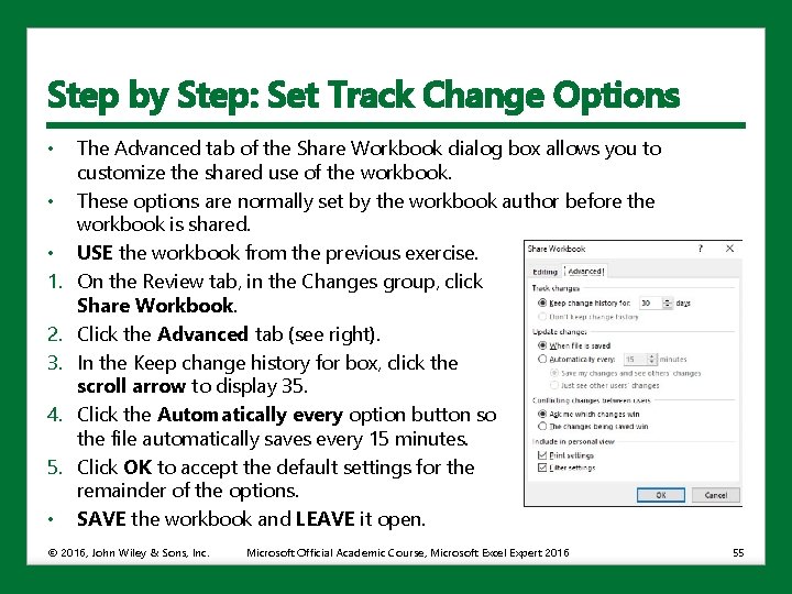
Step by Step: Set Track Change Options • • • 1. 2. 3. 4. 5. • The Advanced tab of the Share Workbook dialog box allows you to customize the shared use of the workbook. These options are normally set by the workbook author before the workbook is shared. USE the workbook from the previous exercise. On the Review tab, in the Changes group, click Share Workbook. Click the Advanced tab (see right). In the Keep change history for box, click the scroll arrow to display 35. Click the Automatically every option button so the file automatically saves every 15 minutes. Click OK to accept the default settings for the remainder of the options. SAVE the workbook and LEAVE it open. © 2016, John Wiley & Sons, Inc. Microsoft Official Academic Course, Microsoft Excel Expert 2016 55

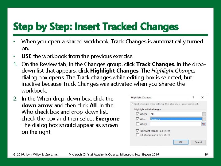
Step by Step: Insert Tracked Changes • When you open a shared workbook, Track Changes is automatically turned on. • USE the workbook from the previous exercise. 1. On the Review tab, in the Changes group, click Track Changes. In the dropdown list that appears, click Highlight Changes. The Highlight Changes dialog box opens. The Track changes while editing box is selected, but inactive because Track Changes was activated when you shared the workbook. 2. In the When drop-down box, click the down arrow and then click All. In the Who check box and drop-down list, check the box and then select Everyone. The dialog box should appear as shown on the right. © 2016, John Wiley & Sons, Inc. Microsoft Official Academic Course, Microsoft Excel Expert 2016 56

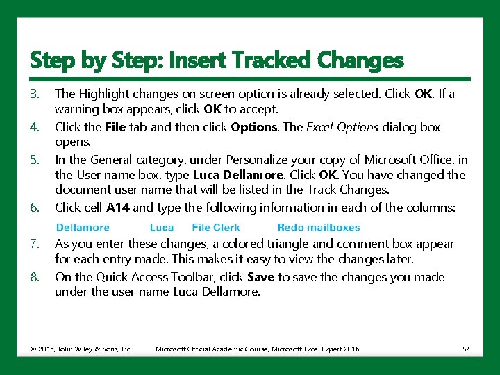
Step by Step: Insert Tracked Changes 3. 4. 5. 6. 7. 8. The Highlight changes on screen option is already selected. Click OK. If a warning box appears, click OK to accept. Click the File tab and then click Options. The Excel Options dialog box opens. In the General category, under Personalize your copy of Microsoft Office, in the User name box, type Luca Dellamore. Click OK. You have changed the document user name that will be listed in the Track Changes. Click cell A 14 and type the following information in each of the columns: As you enter these changes, a colored triangle and comment box appear for each entry made. This makes it easy to view the changes later. On the Quick Access Toolbar, click Save to save the changes you made under the user name Luca Dellamore. © 2016, John Wiley & Sons, Inc. Microsoft Official Academic Course, Microsoft Excel Expert 2016 57

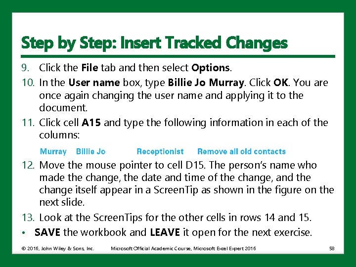
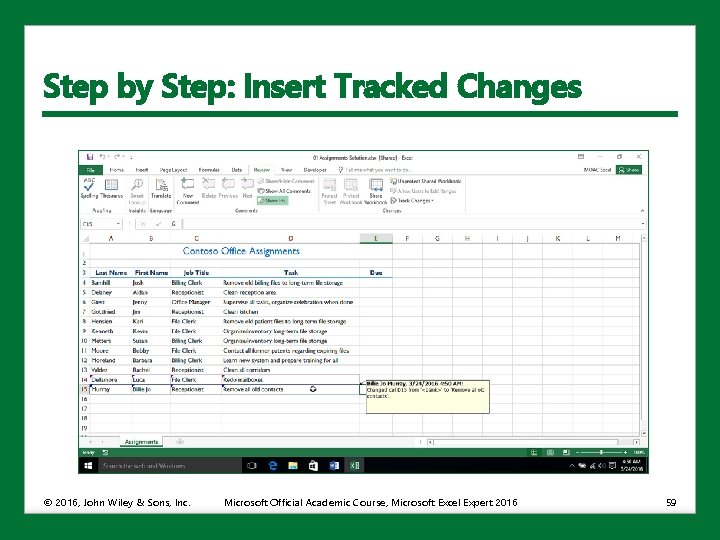
Step by Step: Insert Tracked Changes 9. Click the File tab and then select Options. 10. In the User name box, type Billie Jo Murray. Click OK. You are once again changing the user name and applying it to the document. 11. Click cell A 15 and type the following information in each of the columns: 12. Move the mouse pointer to cell D 15. The person’s name who made the change, the date and time of the change, and the change itself appear in a Screen. Tip as shown in the figure on the next slide. 13. Look at the Screen. Tips for the other cells in rows 14 and 15. • SAVE the workbook and LEAVE it open for the next exercise. © 2016, John Wiley & Sons, Inc. Microsoft Official Academic Course, Microsoft Excel Expert 2016 58

Step by Step: Insert Tracked Changes © 2016, John Wiley & Sons, Inc. Microsoft Official Academic Course, Microsoft Excel Expert 2016 59

Step by Step: Insert Tracked Changes • • On a network, you don’t see changes made by other users until both they and you save your changes. When you work in a network environment, click Share Workbook in the Changes group to see a list of other users who have the workbook open. Sometimes conflicts occur when two users edit a shared workbook and try to save changes that affect the same cell. When the second user tries to save the workbook, Excel displays the Resolve Conflicts dialog box. Depending on the options established, you can either keep your change or accept the change made by the other user. You can also display a list that shows how past conflicts have been resolved. These can be viewed on a separate worksheet that displays the name of the person who made the change, when and where it was made, what data was deleted or replaced, and how conflicts were resolved. © 2016, John Wiley & Sons, Inc. Microsoft Official Academic Course, Microsoft Excel Expert 2016 60

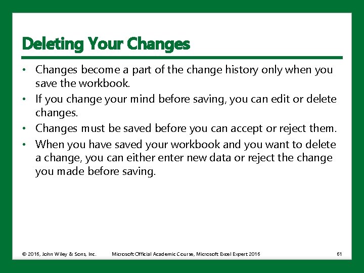
Deleting Your Changes • Changes become a part of the change history only when you save the workbook. • If you change your mind before saving, you can edit or delete changes. • Changes must be saved before you can accept or reject them. • When you have saved your workbook and you want to delete a change, you can either enter new data or reject the change you made before saving. © 2016, John Wiley & Sons, Inc. Microsoft Official Academic Course, Microsoft Excel Expert 2016 61

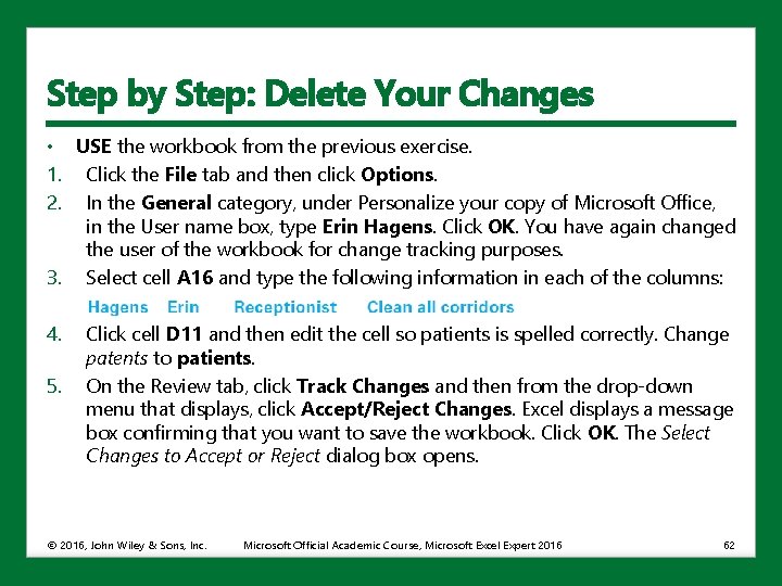
Step by Step: Delete Your Changes • USE the workbook from the previous exercise. 1. Click the File tab and then click Options. 2. In the General category, under Personalize your copy of Microsoft Office, in the User name box, type Erin Hagens. Click OK. You have again changed the user of the workbook for change tracking purposes. 3. Select cell A 16 and type the following information in each of the columns: 4. 5. Click cell D 11 and then edit the cell so patients is spelled correctly. Change patents to patients. On the Review tab, click Track Changes and then from the drop-down menu that displays, click Accept/Reject Changes. Excel displays a message box confirming that you want to save the workbook. Click OK. The Select Changes to Accept or Reject dialog box opens. © 2016, John Wiley & Sons, Inc. Microsoft Official Academic Course, Microsoft Excel Expert 2016 62

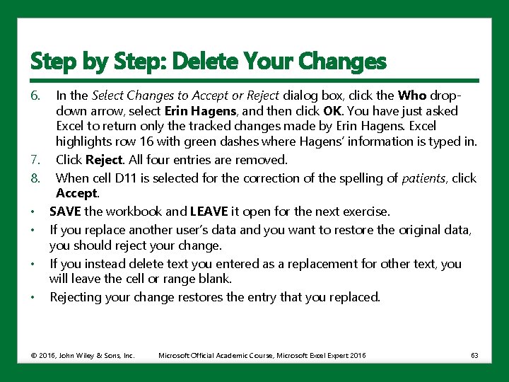
Step by Step: Delete Your Changes 6. In the Select Changes to Accept or Reject dialog box, click the Who dropdown arrow, select Erin Hagens, and then click OK. You have just asked Excel to return only the tracked changes made by Erin Hagens. Excel highlights row 16 with green dashes where Hagens’ information is typed in. 7. Click Reject. All four entries are removed. 8. When cell D 11 is selected for the correction of the spelling of patients, click Accept. • SAVE the workbook and LEAVE it open for the next exercise. • If you replace another user’s data and you want to restore the original data, you should reject your change. • If you instead delete text you entered as a replacement for other text, you will leave the cell or range blank. • Rejecting your change restores the entry that you replaced. © 2016, John Wiley & Sons, Inc. Microsoft Official Academic Course, Microsoft Excel Expert 2016 63

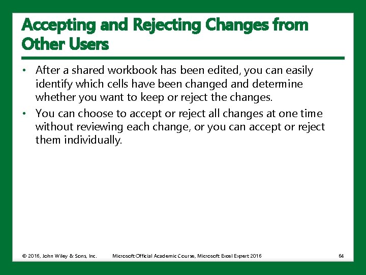
Accepting and Rejecting Changes from Other Users • After a shared workbook has been edited, you can easily identify which cells have been changed and determine whether you want to keep or reject the changes. • You can choose to accept or reject all changes at one time without reviewing each change, or you can accept or reject them individually. © 2016, John Wiley & Sons, Inc. Microsoft Official Academic Course, Microsoft Excel Expert 2016 64

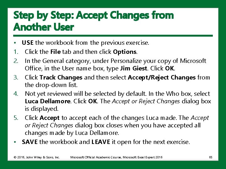
Step by Step: Accept Changes from Another User • USE the workbook from the previous exercise. 1. Click the File tab and then click Options. 2. In the General category, under Personalize your copy of Microsoft Office, in the User name box, type Jim Giest. Click OK. 3. Click Track Changes and then select Accept/Reject Changes from the drop-down list. 4. Not yet reviewed will be selected by default. In the Who box, select Luca Dellamore. Click OK. The Accept or Reject Changes dialog box is displayed. 5. Click Accept to accept each of the changes Luca made. The Accept or Reject Changes dialog box closes when you have accepted all changes made by Luca Dellamore. • SAVE the workbook and LEAVE it open for the next exercise. © 2016, John Wiley & Sons, Inc. Microsoft Official Academic Course, Microsoft Excel Expert 2016 65

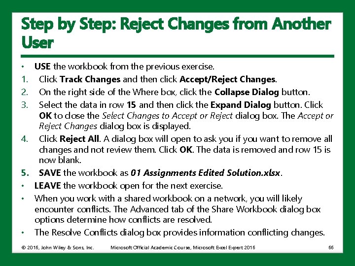
Step by Step: Reject Changes from Another User • USE the workbook from the previous exercise. 1. Click Track Changes and then click Accept/Reject Changes. 2. On the right side of the Where box, click the Collapse Dialog button. 3. Select the data in row 15 and then click the Expand Dialog button. Click OK to close the Select Changes to Accept or Reject dialog box. The Accept or Reject Changes dialog box is displayed. 4. Click Reject All. A dialog box will open to ask you if you want to remove all changes and not review them. Click OK. The data is removed and row 15 is now blank. 5. SAVE the workbook as 01 Assignments Edited Solution. xlsx. • LEAVE the workbook open for the next exercise. • When you work with a shared workbook on a network, you will likely encounter conflicts. The Advanced tab of the Share Workbook dialog box options determine how conflicts are resolved. • The Resolve Conflicts dialog box provides information conflicting changes. © 2016, John Wiley & Sons, Inc. Microsoft Official Academic Course, Microsoft Excel Expert 2016 66

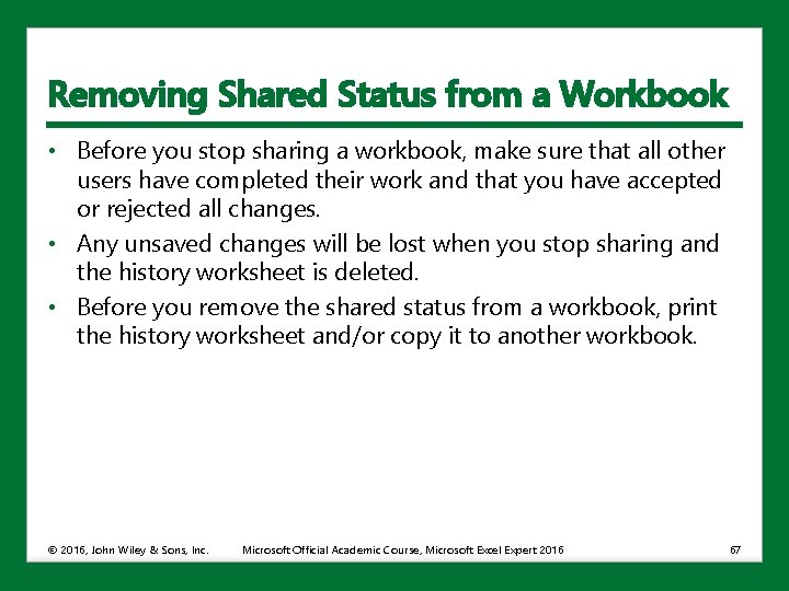
Removing Shared Status from a Workbook • Before you stop sharing a workbook, make sure that all other users have completed their work and that you have accepted or rejected all changes. • Any unsaved changes will be lost when you stop sharing and the history worksheet is deleted. • Before you remove the shared status from a workbook, print the history worksheet and/or copy it to another workbook. © 2016, John Wiley & Sons, Inc. Microsoft Official Academic Course, Microsoft Excel Expert 2016 67

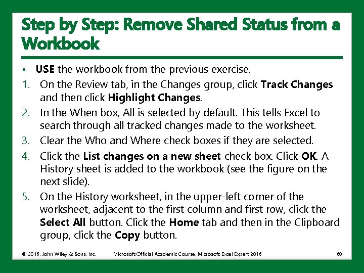
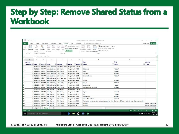
Step by Step: Remove Shared Status from a Workbook • USE the workbook from the previous exercise. 1. On the Review tab, in the Changes group, click Track Changes and then click Highlight Changes. 2. In the When box, All is selected by default. This tells Excel to search through all tracked changes made to the worksheet. 3. Clear the Who and Where check boxes if they are selected. 4. Click the List changes on a new sheet check box. Click OK. A History sheet is added to the workbook (see the figure on the next slide). 5. On the History worksheet, in the upper-left corner of the worksheet, adjacent to the first column and first row, click the Select All button. Click the Home tab and then in the Clipboard group, click the Copy button. © 2016, John Wiley & Sons, Inc. Microsoft Official Academic Course, Microsoft Excel Expert 2016 68

Step by Step: Remove Shared Status from a Workbook © 2016, John Wiley & Sons, Inc. Microsoft Official Academic Course, Microsoft Excel Expert 2016 69

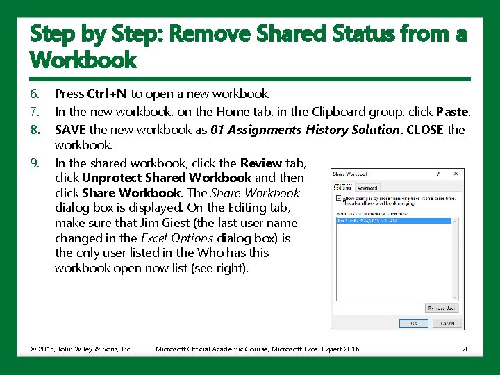
Step by Step: Remove Shared Status from a Workbook 6. 7. 8. 9. Press Ctrl+N to open a new workbook. In the new workbook, on the Home tab, in the Clipboard group, click Paste. SAVE the new workbook as 01 Assignments History Solution. CLOSE the workbook. In the shared workbook, click the Review tab, click Unprotect Shared Workbook and then click Share Workbook. The Share Workbook dialog box is displayed. On the Editing tab, make sure that Jim Giest (the last user name changed in the Excel Options dialog box) is the only user listed in the Who has this workbook open now list (see right). © 2016, John Wiley & Sons, Inc. Microsoft Official Academic Course, Microsoft Excel Expert 2016 70

Step by Step: Remove Shared Status from a Workbook 10. Clear the Allow changes by more than one user at the same time check box. Click OK to close the dialog box. 11. A dialog box opens to prompt you about removing the workbook from shared use. Click Yes to turn off the workbook’s shared status. The word Shared is removed from the title bar and the History worksheet is deleted. 12. Click the File tab and then click Options. 13. In the General category, in the User name box, type your name (or the original user name, before it was changed in this lesson). Click OK. • SAVE the workbook and CLOSE it. • When shared status has been removed from a workbook, changes can be made like they are made in any workbook. • You can, of course, turn change tracking on again, which will automatically share the workbook. © 2016, John Wiley & Sons, Inc. Microsoft Official Academic Course, Microsoft Excel Expert 2016 71

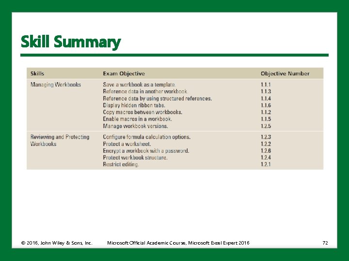
Skill Summary © 2016, John Wiley & Sons, Inc. Microsoft Official Academic Course, Microsoft Excel Expert 2016 72