Microsoft Excel Expert 2016 Lesson 2 Applying Custom

Microsoft Excel Expert 2016 Lesson 2 Applying Custom Formatting and Layouts © 2016, John Wiley & Sons, Inc. Microsoft Official Academic Course, Microsoft Excel Expert 2016 1

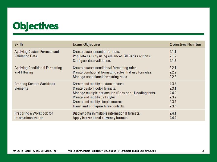
Objectives © 2016, John Wiley & Sons, Inc. Microsoft Official Academic Course, Microsoft Excel Expert 2016 2

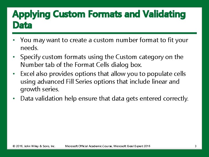
Applying Custom Formats and Validating Data • You may want to create a custom number format to fit your needs. • Specify custom formats using the Custom category on the Number tab of the Format Cells dialog box. • Excel also provides options that allow you to populate cells using advanced Fill Series options that include linear and growth series. • Data validation help ensure that data gets entered correctly. © 2016, John Wiley & Sons, Inc. Microsoft Official Academic Course, Microsoft Excel Expert 2016 3

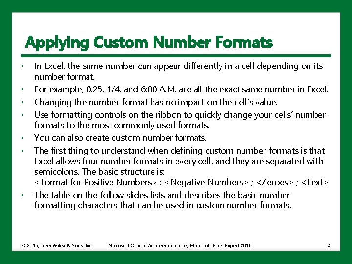
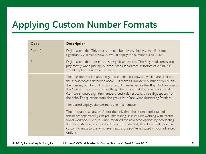
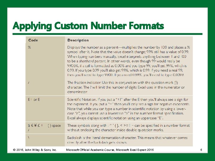
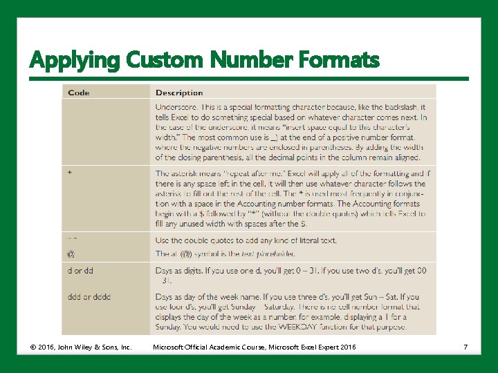
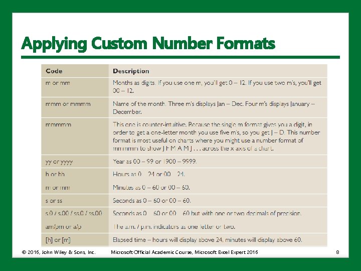
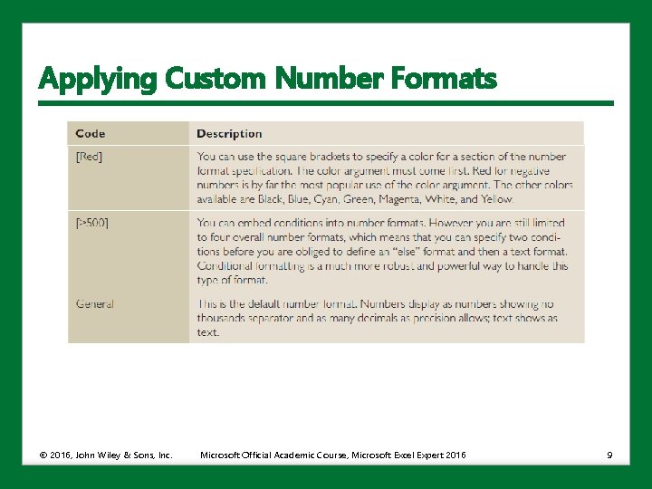
Applying Custom Number Formats • • In Excel, the same number can appear differently in a cell depending on its number format. For example, 0. 25, 1/4, and 6: 00 A. M. are all the exact same number in Excel. Changing the number format has no impact on the cell’s value. Use formatting controls on the ribbon to quickly change your cells’ number formats to the most commonly used formats. You can also create custom number formats. The first thing to understand when defining custom number formats is that Excel allows four number formats in every cell, and they are separated with semicolons. The basic structure is: <Format for Positive Numbers> ; <Negative Numbers> ; <Zeroes> ; <Text> The table on the follow slides lists and describes the basic number formatting characters that can be used in custom number formats. © 2016, John Wiley & Sons, Inc. Microsoft Official Academic Course, Microsoft Excel Expert 2016 4

Applying Custom Number Formats © 2016, John Wiley & Sons, Inc. Microsoft Official Academic Course, Microsoft Excel Expert 2016 5

Applying Custom Number Formats © 2016, John Wiley & Sons, Inc. Microsoft Official Academic Course, Microsoft Excel Expert 2016 6

Applying Custom Number Formats © 2016, John Wiley & Sons, Inc. Microsoft Official Academic Course, Microsoft Excel Expert 2016 7

Applying Custom Number Formats © 2016, John Wiley & Sons, Inc. Microsoft Official Academic Course, Microsoft Excel Expert 2016 8

Applying Custom Number Formats © 2016, John Wiley & Sons, Inc. Microsoft Official Academic Course, Microsoft Excel Expert 2016 9

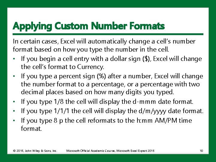
Applying Custom Number Formats In certain cases, Excel will automatically change a cell’s number format based on how you type the number in the cell. • If you begin a cell entry with a dollar sign ($), Excel will change the cell’s format to Currency. • If you type a percent sign (%) after a number, Excel will change the number format to a percentage, or a percentage with two decimal places based on how many digits you typed. • If you type 1/8 the cell will display the d-mmm date format. • If you type 1/1/1 the cell will display the d/m/yyyy date format. • If you type 8 p the cell reformats to the h: mm AM/PM time format. © 2016, John Wiley & Sons, Inc. Microsoft Official Academic Course, Microsoft Excel Expert 2016 10

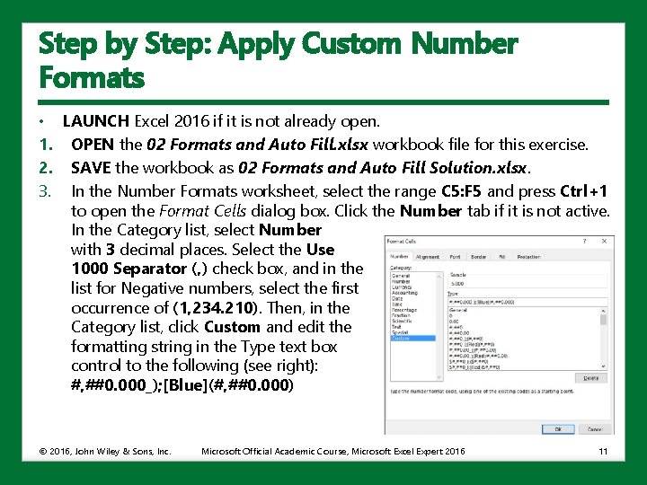
Step by Step: Apply Custom Number Formats • LAUNCH Excel 2016 if it is not already open. 1. OPEN the 02 Formats and Auto Fill. xlsx workbook file for this exercise. 2. SAVE the workbook as 02 Formats and Auto Fill Solution. xlsx. 3. In the Number Formats worksheet, select the range C 5: F 5 and press Ctrl+1 to open the Format Cells dialog box. Click the Number tab if it is not active. In the Category list, select Number with 3 decimal places. Select the Use 1000 Separator (, ) check box, and in the list for Negative numbers, select the first occurrence of (1, 234. 210). Then, in the Category list, click Custom and edit the formatting string in the Type text box control to the following (see right): #, ##0. 000_); [Blue](#, ##0. 000) © 2016, John Wiley & Sons, Inc. Microsoft Official Academic Course, Microsoft Excel Expert 2016 11

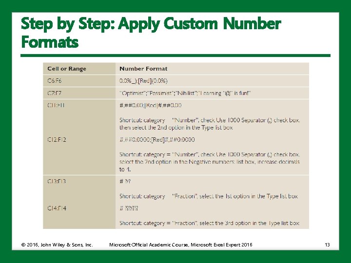
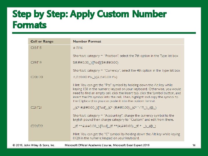
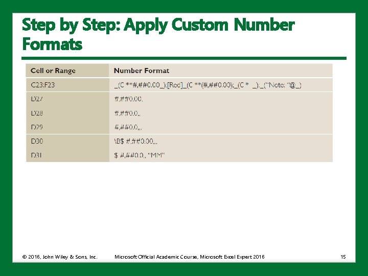
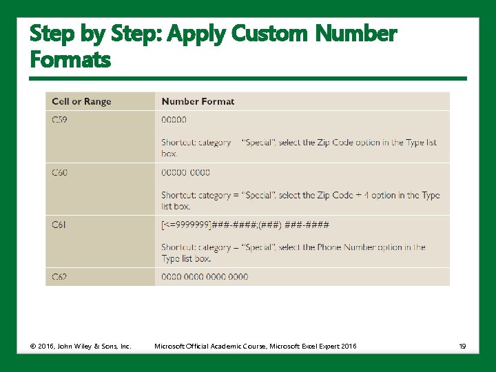
Step by Step: Apply Custom Number Formats 4. Click OK. Use the Number tab in the Format Cells dialog box to set the number formats in the ranges listed in the table on the next slides, per the specification indicated. In all instances you can directly select the Custom category and type in the number format. However you can often “jump start” the process by using a predefined number format first and then switching to the Custom category and making any final edits. If available, a shortcut that will default to the desired format or get you close is shown below the desired number format. After trying each shortcut, select the Custom category to make sure you have the desired format and make any needed edits there. © 2016, John Wiley & Sons, Inc. Microsoft Official Academic Course, Microsoft Excel Expert 2016 12

Step by Step: Apply Custom Number Formats © 2016, John Wiley & Sons, Inc. Microsoft Official Academic Course, Microsoft Excel Expert 2016 13

Step by Step: Apply Custom Number Formats © 2016, John Wiley & Sons, Inc. Microsoft Official Academic Course, Microsoft Excel Expert 2016 14

Step by Step: Apply Custom Number Formats © 2016, John Wiley & Sons, Inc. Microsoft Official Academic Course, Microsoft Excel Expert 2016 15

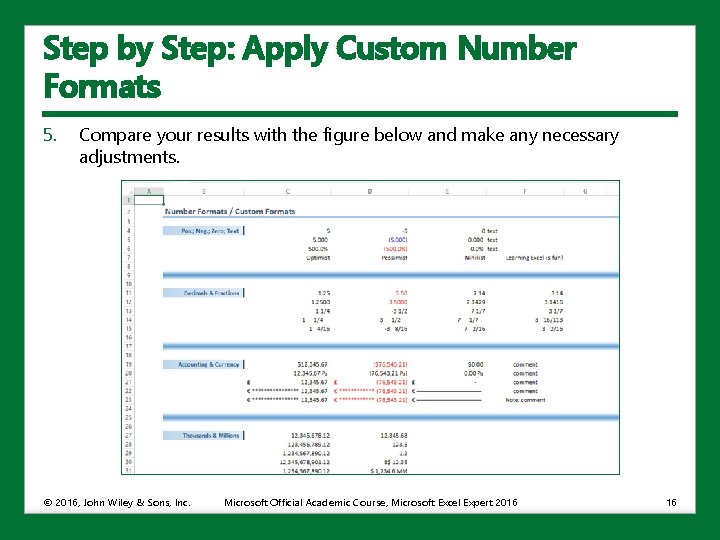
Step by Step: Apply Custom Number Formats 5. Compare your results with the figure below and make any necessary adjustments. © 2016, John Wiley & Sons, Inc. Microsoft Official Academic Course, Microsoft Excel Expert 2016 16

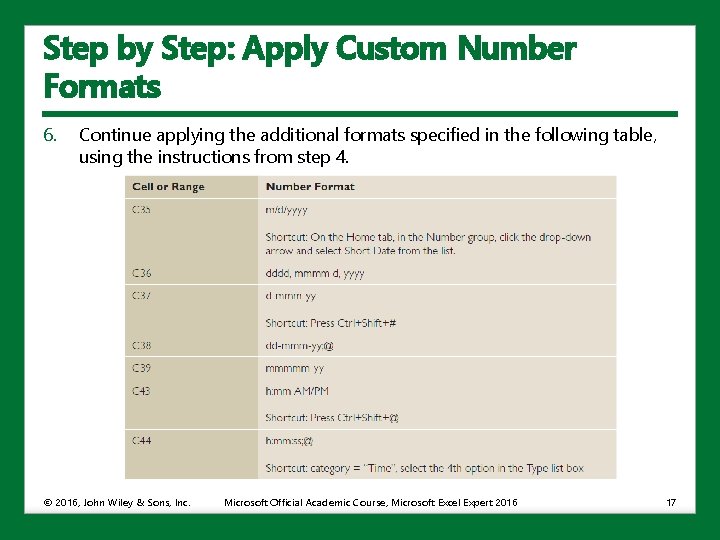
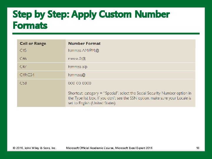
Step by Step: Apply Custom Number Formats 6. Continue applying the additional formats specified in the following table, using the instructions from step 4. © 2016, John Wiley & Sons, Inc. Microsoft Official Academic Course, Microsoft Excel Expert 2016 17

Step by Step: Apply Custom Number Formats © 2016, John Wiley & Sons, Inc. Microsoft Official Academic Course, Microsoft Excel Expert 2016 18

Step by Step: Apply Custom Number Formats © 2016, John Wiley & Sons, Inc. Microsoft Official Academic Course, Microsoft Excel Expert 2016 19

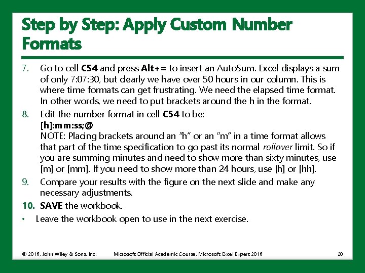
Step by Step: Apply Custom Number Formats 7. Go to cell C 54 and press Alt+= to insert an Auto. Sum. Excel displays a sum of only 7: 07: 30, but clearly we have over 50 hours in our column. This is where time formats can get frustrating. We need the elapsed time format. In other words, we need to put brackets around the h in the format. 8. Edit the number format in cell C 54 to be: [h]: mm: ss; @ NOTE: Placing brackets around an “h” or an “m” in a time format allows that part of the time specification to go past its normal rollover limit. So if you are summing minutes and need to show more than sixty minutes, use [m] or [mm]. If you need to show more than 24 hours, use [h] or [hh]. 9. Compare your results with the figure on the next slide and make any necessary adjustments. 10. SAVE the workbook. • Leave the workbook open to use in the next exercise. © 2016, John Wiley & Sons, Inc. Microsoft Official Academic Course, Microsoft Excel Expert 2016 20

Step by Step: Apply Custom Number Formats © 2016, John Wiley & Sons, Inc. Microsoft Official Academic Course, Microsoft Excel Expert 2016 21

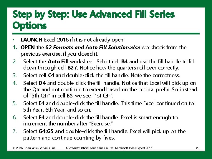
Step by Step: Use Advanced Fill Series Options • LAUNCH Excel 2016 if it is not already open. 1. OPEN the 02 Formats and Auto Fill Solution. xlsx workbook from the previous exercise, if you closed it. 2. Select the Auto Fill worksheet. Select cell B 4 and use the fill handle to fill down through cell B 27. Notice how the quarters roll over correctly. 3. Select cell C 4 and double-click the fill handle. Note the correctness. 4. Select D 4 and double-click the fill handle. Notice that Excel will pick up on the Qtr and not continue to extend based on the ordinal prefix. So, instead of “ 5 th Qtr” in cell B 8, we see “ 1 st Qtr”. 5. Select E 4 and double-click the fill handle. This time Excel continued on to 5 th Year, 6 th Year, and so on. 6. Select F 4 and double-click the fill handle. Excel is smart enough to increment the number after “Exercise. ” 7. Select G 4: G 5 and double-click the fill handle. Excel will pick up on the pattern and continue counting by fives. © 2016, John Wiley & Sons, Inc. Microsoft Official Academic Course, Microsoft Excel Expert 2016 22

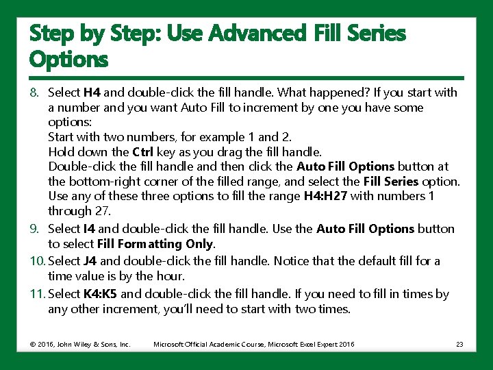
Step by Step: Use Advanced Fill Series Options 8. Select H 4 and double-click the fill handle. What happened? If you start with a number and you want Auto Fill to increment by one you have some options: Start with two numbers, for example 1 and 2. Hold down the Ctrl key as you drag the fill handle. Double-click the fill handle and then click the Auto Fill Options button at the bottom-right corner of the filled range, and select the Fill Series option. Use any of these three options to fill the range H 4: H 27 with numbers 1 through 27. 9. Select I 4 and double-click the fill handle. Use the Auto Fill Options button to select Fill Formatting Only. 10. Select J 4 and double-click the fill handle. Notice that the default fill for a time value is by the hour. 11. Select K 4: K 5 and double-click the fill handle. If you need to fill in times by any other increment, you’ll need to start with two times. © 2016, John Wiley & Sons, Inc. Microsoft Official Academic Course, Microsoft Excel Expert 2016 23

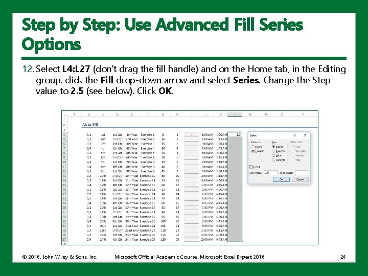
Step by Step: Use Advanced Fill Series Options 12. Select L 4: L 27 (don’t drag the fill handle) and on the Home tab, in the Editing group, click the Fill drop-down arrow and select Series. Change the Step value to 2. 5 (see below). Click OK. © 2016, John Wiley & Sons, Inc. Microsoft Official Academic Course, Microsoft Excel Expert 2016 24

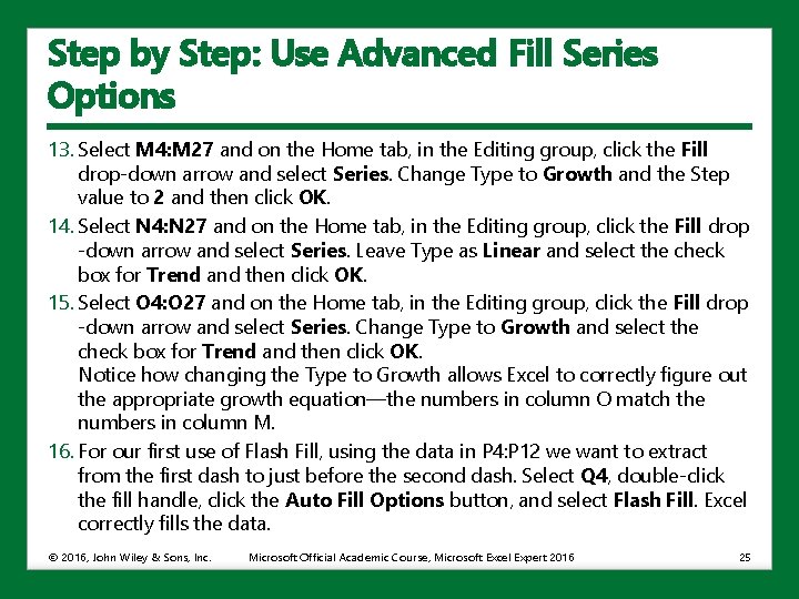
Step by Step: Use Advanced Fill Series Options 13. Select M 4: M 27 and on the Home tab, in the Editing group, click the Fill drop-down arrow and select Series. Change Type to Growth and the Step value to 2 and then click OK. 14. Select N 4: N 27 and on the Home tab, in the Editing group, click the Fill drop -down arrow and select Series. Leave Type as Linear and select the check box for Trend and then click OK. 15. Select O 4: O 27 and on the Home tab, in the Editing group, click the Fill drop -down arrow and select Series. Change Type to Growth and select the check box for Trend and then click OK. Notice how changing the Type to Growth allows Excel to correctly figure out the appropriate growth equation—the numbers in column O match the numbers in column M. 16. For our first use of Flash Fill, using the data in P 4: P 12 we want to extract from the first dash to just before the second dash. Select Q 4, double-click the fill handle, click the Auto Fill Options button, and select Flash Fill. Excel correctly fills the data. © 2016, John Wiley & Sons, Inc. Microsoft Official Academic Course, Microsoft Excel Expert 2016 25

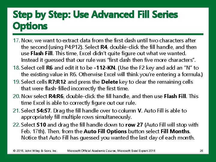
Step by Step: Use Advanced Fill Series Options 17. Now, we want to extract data from the first dash until two characters after the second (using P 4: P 12). Select R 4, double-click the fill handle, and then use Flash Fill. This time, Excel didn’t quite figure out what we wanted. Instead it guessed that our rule was “first dash then five more characters”. 18. Select cell R 6 and edit it to be -112 -KN. (Use the F 2 key and add an “N” to the existing value in R 6. Otherwise Excel will think you’re entering a formula. ) 19. Select cells R 7: R 12 and press the Delete key to clear the remaining cells that were flash-filled incorrectly the first time. 20. Now select R 4: R 6, double-click the fill handle, and then use Flash Fill. This time Excel is able to correctly figure out our rule. 21. Select S 4: S 7. Drag the fill handle over to column V. Auto Fill is able to appropriately fill multiple rows simultaneously. 22. Select S 10 and drag the fill handle down to row 27 (Auto Fill will stop with Feb. 17 th). Then, from the Auto Fill Options button select Fill Months. Notice that Auto Fill has guessed you wanted the last day of each month. © 2016, John Wiley & Sons, Inc. Microsoft Official Academic Course, Microsoft Excel Expert 2016 26

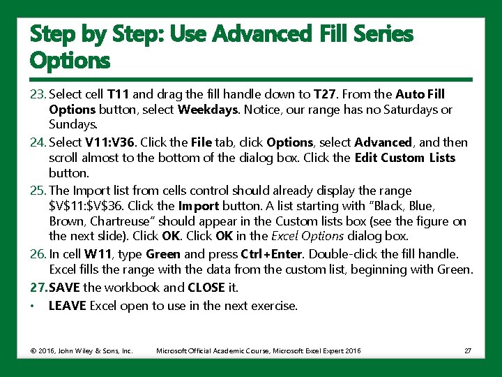
Step by Step: Use Advanced Fill Series Options 23. Select cell T 11 and drag the fill handle down to T 27. From the Auto Fill Options button, select Weekdays. Notice, our range has no Saturdays or Sundays. 24. Select V 11: V 36. Click the File tab, click Options, select Advanced, and then scroll almost to the bottom of the dialog box. Click the Edit Custom Lists button. 25. The Import list from cells control should already display the range $V$11: $V$36. Click the Import button. A list starting with “Black, Blue, Brown, Chartreuse” should appear in the Custom lists box (see the figure on the next slide). Click OK in the Excel Options dialog box. 26. In cell W 11, type Green and press Ctrl+Enter. Double-click the fill handle. Excel fills the range with the data from the custom list, beginning with Green. 27. SAVE the workbook and CLOSE it. • LEAVE Excel open to use in the next exercise. © 2016, John Wiley & Sons, Inc. Microsoft Official Academic Course, Microsoft Excel Expert 2016 27

Step by Step: Use Advanced Fill Series Options © 2016, John Wiley & Sons, Inc. Microsoft Official Academic Course, Microsoft Excel Expert 2016 28

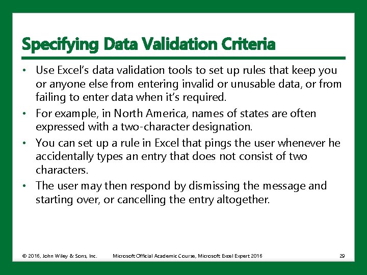
Specifying Data Validation Criteria • Use Excel’s data validation tools to set up rules that keep you or anyone else from entering invalid or unusable data, or from failing to enter data when it’s required. • For example, in North America, names of states are often expressed with a two-character designation. • You can set up a rule in Excel that pings the user whenever he accidentally types an entry that does not consist of two characters. • The user may then respond by dismissing the message and starting over, or cancelling the entry altogether. © 2016, John Wiley & Sons, Inc. Microsoft Official Academic Course, Microsoft Excel Expert 2016 29

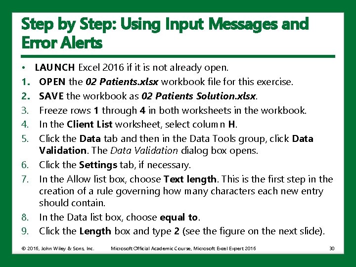
Step by Step: Using Input Messages and Error Alerts • 1. 2. 3. 4. 5. 6. 7. 8. 9. LAUNCH Excel 2016 if it is not already open. OPEN the 02 Patients. xlsx workbook file for this exercise. SAVE the workbook as 02 Patients Solution. xlsx. Freeze rows 1 through 4 in both worksheets in the workbook. In the Client List worksheet, select column H. Click the Data tab and then in the Data Tools group, click Data Validation. The Data Validation dialog box opens. Click the Settings tab, if necessary. In the Allow list box, choose Text length. This is the first step in the creation of a rule governing how many characters each new entry should contain. In the Data list box, choose equal to. Click the Length box and type 2 (see the figure on the next slide). © 2016, John Wiley & Sons, Inc. Microsoft Official Academic Course, Microsoft Excel Expert 2016 30

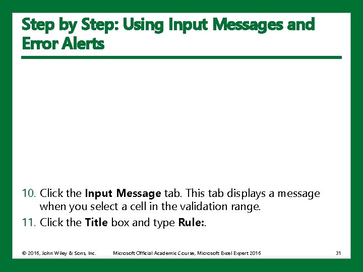
Step by Step: Using Input Messages and Error Alerts 10. Click the Input Message tab. This tab displays a message when you select a cell in the validation range. 11. Click the Title box and type Rule: . © 2016, John Wiley & Sons, Inc. Microsoft Official Academic Course, Microsoft Excel Expert 2016 31

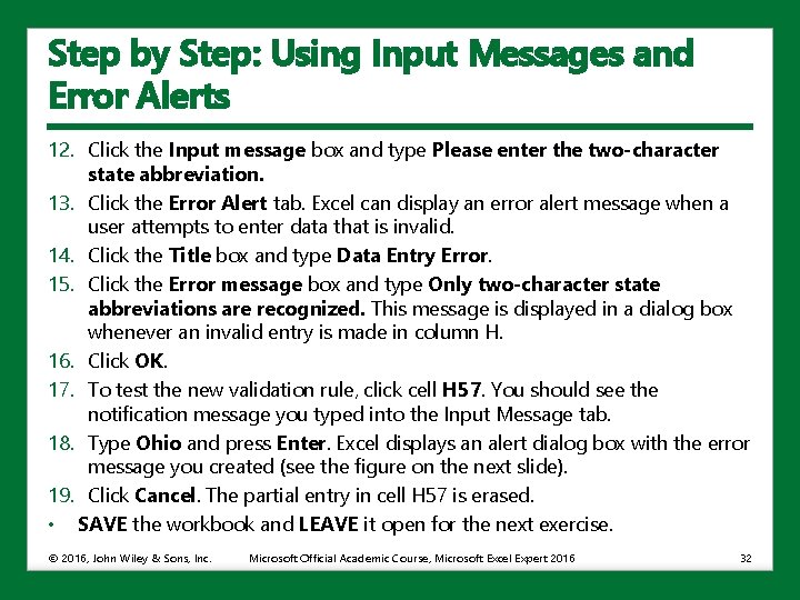
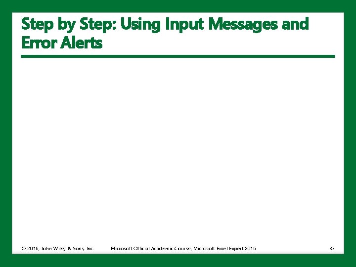
Step by Step: Using Input Messages and Error Alerts 12. Click the Input message box and type Please enter the two-character state abbreviation. 13. Click the Error Alert tab. Excel can display an error alert message when a user attempts to enter data that is invalid. 14. Click the Title box and type Data Entry Error. 15. Click the Error message box and type Only two-character state abbreviations are recognized. This message is displayed in a dialog box whenever an invalid entry is made in column H. 16. Click OK. 17. To test the new validation rule, click cell H 57. You should see the notification message you typed into the Input Message tab. 18. Type Ohio and press Enter. Excel displays an alert dialog box with the error message you created (see the figure on the next slide). 19. Click Cancel. The partial entry in cell H 57 is erased. • SAVE the workbook and LEAVE it open for the next exercise. © 2016, John Wiley & Sons, Inc. Microsoft Official Academic Course, Microsoft Excel Expert 2016 32

Step by Step: Using Input Messages and Error Alerts © 2016, John Wiley & Sons, Inc. Microsoft Official Academic Course, Microsoft Excel Expert 2016 33

Step by Step: Using Lists for Data Validation Criteria • Many databases includes fields that allow a specified number of valid entries. • In data entry, it’s easy for someone to slip and type an invalid entry. • You can preempt events like this by building a rule that restricts entry to a handful of valid entries. • LAUNCH Excel 2016 if it is not already open. 1. OPEN the 02 Patients Solution. xlsx workbook from the previous exercise, if you closed it. 2. Click the Patient List sheet tab. 3. Select column B. 4. Click the Data tab and then in the Data Tools group, click Data Validation. 5. In the Data Validation dialog box, click the Settings tab. © 2016, John Wiley & Sons, Inc. Microsoft Official Academic Course, Microsoft Excel Expert 2016 34

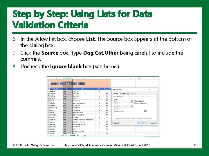
Step by Step: Using Lists for Data Validation Criteria 6. In the Allow list box, choose List. The Source box appears at the bottom of the dialog box. 7. Click the Source box. Type Dog, Cat, Other being careful to include the commas. 8. Uncheck the Ignore blank box (see below). © 2016, John Wiley & Sons, Inc. Microsoft Official Academic Course, Microsoft Excel Expert 2016 35

Step by Step: Using Lists for Data Validation Criteria 9. Click the Input Message tab. Click the Title box and type Rule: . Then, click in the Input message box and type Choose from Dog, Cat, or Other. 10. Click OK. Now anyone entering a new patient into the database must specify the animal type from a drop-down list in column B. We’ll test this validation rule later in this exercise. 11. Next, we’ll specify a validation list for another column in the database. Select column E (Owner #). 12. In the Data Tools group, click Data Validation. 13. Click the Settings tab. In the Allow list box, click List. 14. On the right side of the Source box, click the Collapse Dialog button. © 2016, John Wiley & Sons, Inc. Microsoft Official Academic Course, Microsoft Excel Expert 2016 36

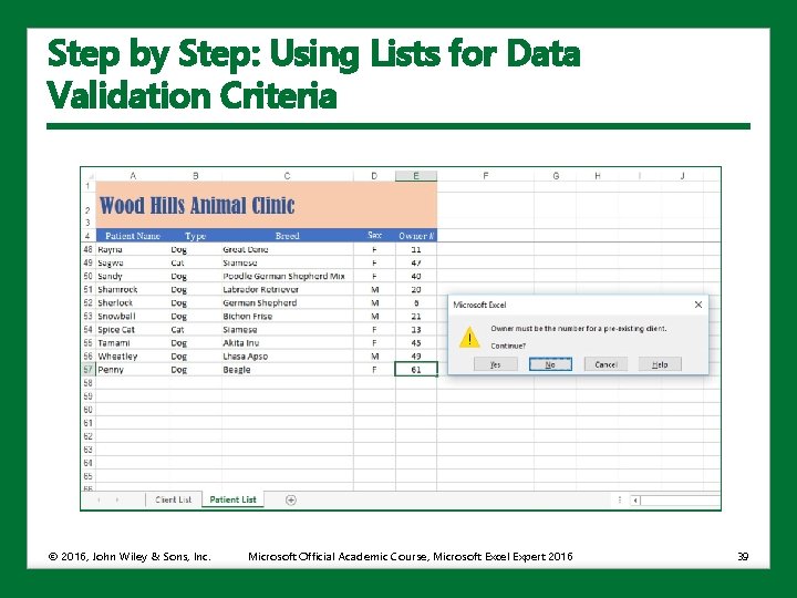
Step by Step: Using Lists for Data Validation Criteria 15. With the Data Validation dialog box collapsed, click the Client List worksheet tab. 16. Select column A (Client #). 17. At the end of the Source box, click the Expand Dialog button. The full dialog box returns, and the Source box should now read =’Client list’!$A: $A. 18. Uncheck the Ignore blank and In-cell dropdown boxes. 19. Click the Error Alert tab. Choose Warning from the Style box. 20. In the Error message box, type Owner must be the number for a pre-existing client. 21. Click OK. Now the Owner # column may contain only numbers for clients who appear in the Client # column of the Client List worksheet. © 2016, John Wiley & Sons, Inc. Microsoft Official Academic Course, Microsoft Excel Expert 2016 37

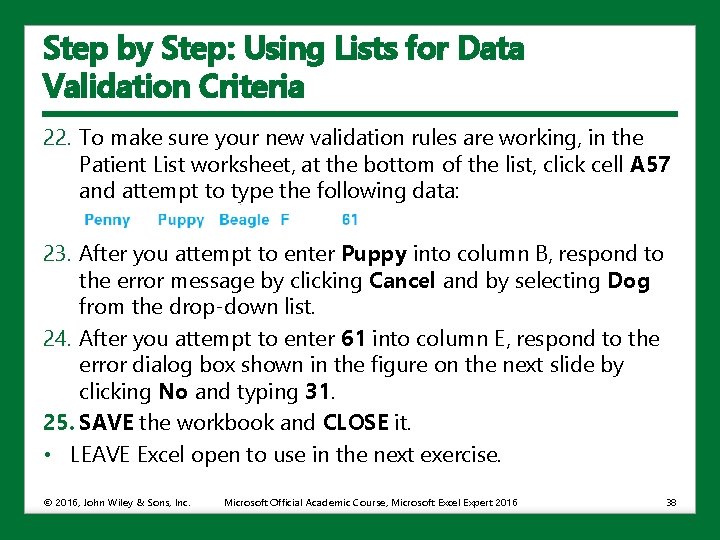
Step by Step: Using Lists for Data Validation Criteria 22. To make sure your new validation rules are working, in the Patient List worksheet, at the bottom of the list, click cell A 57 and attempt to type the following data: 23. After you attempt to enter Puppy into column B, respond to the error message by clicking Cancel and by selecting Dog from the drop-down list. 24. After you attempt to enter 61 into column E, respond to the error dialog box shown in the figure on the next slide by clicking No and typing 31. 25. SAVE the workbook and CLOSE it. • LEAVE Excel open to use in the next exercise. © 2016, John Wiley & Sons, Inc. Microsoft Official Academic Course, Microsoft Excel Expert 2016 38

Step by Step: Using Lists for Data Validation Criteria © 2016, John Wiley & Sons, Inc. Microsoft Official Academic Course, Microsoft Excel Expert 2016 39

Applying Conditional Formatting and Filtering • Conditional formatting is a powerful Excel feature that enables you to specify how cells that meet a given condition should be displayed. • This means that Excel applies formatting, based on established criteria. • When you analyze data, you often ask questions, such as: • Who are the highest performing students in the gradebook? • Which sales representatives exceeded their sales goals and in which quarters? • In what months were revenues highest or lowest? • Conditional formatting helps answer such questions by highlighting pertinent cells or ranges of cells. • You can even establish multiple conditional formatting rules for a data range. © 2016, John Wiley & Sons, Inc. Microsoft Official Academic Course, Microsoft Excel Expert 2016 40

Step by Step: Apply Conditional Formatting • To apply a specific conditional format, use the Conditional Formatting menu in the Styles group on the Home tab and select one of the many options provided. • LAUNCH Excel if it is not already running. 1. OPEN the 02 Conditional Formatting. xlsx workbook file for this exercise. 2. SAVE the workbook as 02 Conditional Formatting Solution. xlsx. 3. In the Format 1 worksheet, select D 5: O 9. You will apply conditional formatting to all cells in this range. © 2016, John Wiley & Sons, Inc. Microsoft Official Academic Course, Microsoft Excel Expert 2016 41

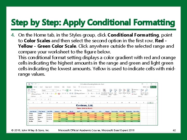
Step by Step: Apply Conditional Formatting 4. On the Home tab, in the Styles group, click Conditional Formatting, point to Color Scales and then select the second option in the first row, Red Yellow - Green Color Scale. Click anywhere outside the selected range and compare your worksheet to the figure below. This conditional format setting displays a color gradient with red and orange cells indicating the highest amounts in the range and green and light green cells indicating the lowest amounts. Yellow is used to indicate cells with midrange values. © 2016, John Wiley & Sons, Inc. Microsoft Official Academic Course, Microsoft Excel Expert 2016 42

Step by Step: Apply Conditional Formatting 5. Click Undo in the Quick Access Toolbar to remove the conditional formatting that you applied in the previous step. 6. Select D 5: O 9 again, if necessary. 7. On the Home tab, in the Styles group, click Conditional Formatting, point to Highlight Cells Rules, and then select Greater Than. The Greater Than dialog box opens. 8. In the Format cells that are GREATER THAN box, type 600. © 2016, John Wiley & Sons, Inc. Microsoft Official Academic Course, Microsoft Excel Expert 2016 43

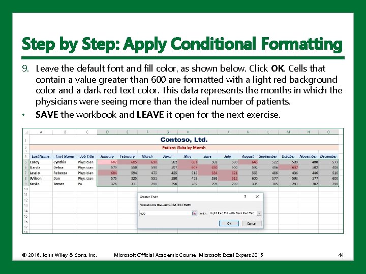
Step by Step: Apply Conditional Formatting 9. Leave the default font and fill color, as shown below. Click OK. Cells that contain a value greater than 600 are formatted with a light red background color and a dark red text color. This data represents the months in which the physicians were seeing more than the ideal number of patients. • SAVE the workbook and LEAVE it open for the next exercise. © 2016, John Wiley & Sons, Inc. Microsoft Official Academic Course, Microsoft Excel Expert 2016 44

Using Formulas in Conditional Formatting Rules • You can use preset rules provided by Excel to apply conditional formatting to data or customize rules for your particular needs. • The Excel Rules Manager gives you even greater control over rules by enabling you to: • Set the order of multiple rules • Fine-tune rule settings • Use formulas that you enter to determine which cells to format © 2016, John Wiley & Sons, Inc. Microsoft Official Academic Course, Microsoft Excel Expert 2016 45

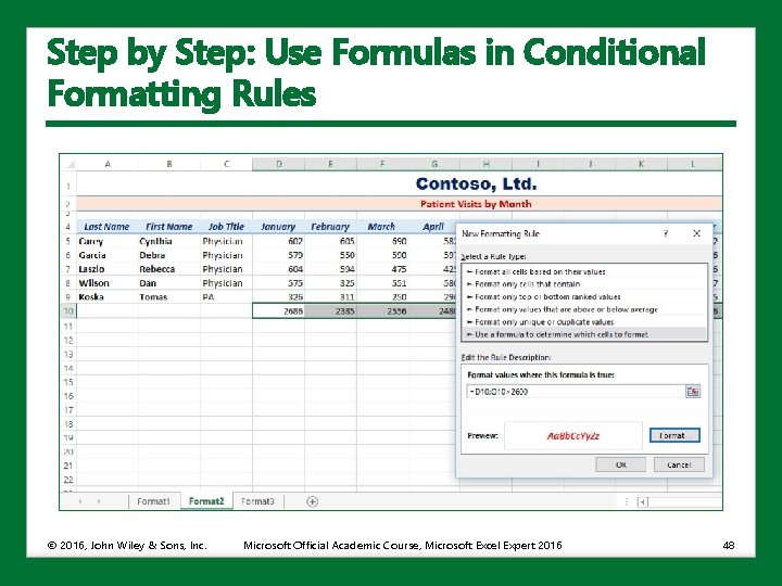
Step by Step: Use Formulas in Conditional Formatting Rules • LAUNCH Excel 2016 if it is not already open. 1. OPEN the 02 Conditional Formatting Solution. xlsx workbook from the previous exercise, if you closed it. 2. Click the Format 2 sheet tab. 3. Select the range D 5: O 9. On the Home tab, in the Editing group, click Auto. Sum. Monthly totals are added to row 10. 4. Select D 10: O 10. In the Font group, click the Borders button arrow and select Top and Double Bottom Border. 5. With D 10: O 10 still selected, in the Styles group, click Conditional Formatting and then select New Rule. The New Formatting Rule dialog box opens. 6. In the Select a Rule Type list, click Use a formula to determine which cells to format. © 2016, John Wiley & Sons, Inc. Microsoft Official Academic Course, Microsoft Excel Expert 2016 46

Step by Step: Use Formulas in Conditional Formatting Rules 7. In the Edit the Rule Description section, click in the Format values where this formula is true box and then type =D 10: O 10>2600. Be sure to precede the formula with an equal sign. 8. Click the Format button. In the Format Cells dialog box, select Red from the Color drop-down palette. Click Bold Italic in the Font style list and then click OK. The Preview box shows the formatting that will be applied to cells where the formula evaluates to True (see the figure on the next slide). 9. Click OK to apply the rule. Four of the five months—January, June, July, and August—display the conditional formatting, indicating that the total number of patients exceeded 2, 600 in these months. • SAVE the workbook and LEAVE it open for the next exercise. © 2016, John Wiley & Sons, Inc. Microsoft Official Academic Course, Microsoft Excel Expert 2016 47

Step by Step: Use Formulas in Conditional Formatting Rules © 2016, John Wiley & Sons, Inc. Microsoft Official Academic Course, Microsoft Excel Expert 2016 48

Managing Conditional Formatting Rules • The Excel Rules Manager enables you to create, modify, apply, remove, and manage conditional formatting, including multiple criteria. • You can apply a single rule or multiple rules, and you can modify preset rules to display formats however you like. © 2016, John Wiley & Sons, Inc. Microsoft Official Academic Course, Microsoft Excel Expert 2016 49

Step by Step: Manage Conditional Formatting Rules • LAUNCH Excel 2016 if it is not already open. 1. OPEN the 02 Conditional Formatting Solution. xlsx workbook from the previous exercise, if you closed it. 2. Click the Format 3 sheet tab. 3. Select the range D 5: O 9. 4. On the Home tab, in the Styles group, open the Conditional Formatting menu, and select Clear Rules > Clear Rules from Selected Cells to ensure that no formatting is specified for these cells. 5. Open the Conditional Formatting menu again and select Manage Rules. The Conditional Formatting Rules Manager dialog box opens. © 2016, John Wiley & Sons, Inc. Microsoft Official Academic Course, Microsoft Excel Expert 2016 50

Step by Step: Manage Conditional Formatting Rules 6. Click the Show formatting rules for arrow and select Sheet: Format 1 to view the rule you applied in the Format 1 worksheet. Then click the Show formatting rules for arrow and select Sheet: Format 2 to see the rule applied to that worksheet. Finally, return to the Current Selection setting in the drop-down list. 7. Click the New Rule button. In the New Formatting Rule dialog box, select Format only top or bottom ranked values. 8. In the Edit the Rule Description section, click the % of the selected range check box. 9. Click the Format button. The Format Cells dialog box opens. 10. Click the Fill tab and then select the light orange color box, the sixth color in the third row. Click OK twice. © 2016, John Wiley & Sons, Inc. Microsoft Official Academic Course, Microsoft Excel Expert 2016 51

Step by Step: Manage Conditional Formatting Rules 11. In the Conditional Formatting Rules Manager dialog box, click the New Rule button again. 12. In the New Formatting Rule dialog box, select Format only top or bottom ranked values. 13. In the Edit the Rule Description section, in the first drop-down list on the left, select Bottom and then click the % of the selected range check box. 14. Click the Format button. 15. In the Format Cells dialog box, click the light green background color on the third row of the Fill tab and then click OK twice. Both rules now display in the dialog box (see right). © 2016, John Wiley & Sons, Inc. Microsoft Official Academic Course, Microsoft Excel Expert 2016 52

Step by Step: Manage Conditional Formatting Rules 16. Click OK and then click outside of the selected range. The Rules Manager applies the two rules to the selected cells, as shown below. This formatting enables you to easily see the top 10 percent and bottom 10 percent of values in the range. 17. SAVE the workbook and CLOSE it. • LEAVE Excel open to use in the next exercise. © 2016, John Wiley & Sons, Inc. Microsoft Official Academic Course, Microsoft Excel Expert 2016 53

Step by Step: Manage Conditional Formatting Rules • You can display the Rules Manager to see what rules are in effect for the worksheet and apply those rules at an appropriate time. • From the Conditional Formatting Rules Manager dialog box, you can: • Add new rules • Edit existing rules • Delete one or all of the rules • Apply all the rules • Apply specific rules to analyze the data • Formatting is visible when the Conditional Formatting Rules Manager dialog box is open. • You can experiment with the formats you want to apply and the order in which they are applied. © 2016, John Wiley & Sons, Inc. Microsoft Official Academic Course, Microsoft Excel Expert 2016 54

Creating Custom Workbook Elements • In Excel, you can create and modify custom workbook elements such as: • Themes • Color formats • Font formats • Cell styles • Macros • Form controls • Options for customizing cell styles, themes, colors, and fonts are located on the Home and Page Layout tabs of the ribbon. • You must add the Developer tab to the ribbon to access commands for creating macros and inserting form controls. © 2016, John Wiley & Sons, Inc. Microsoft Official Academic Course, Microsoft Excel Expert 2016 55

Creating and Modifying Custom Themes • A document theme is a predefined set of colors, fonts, and effects that can be applied to a workbook. • You can use document themes to easily format an entire document and give it a fresh, professional look. Themes are also used in other Office applications, which allows you to give all your Office documents a uniform look. • Excel has several predefined document themes. • When you apply a theme to a workbook, the colors, fonts, and effects contained within that theme replace any styles that were already applied to cells or ranges. • You can modify predefined themes to create a custom theme. © 2016, John Wiley & Sons, Inc. Microsoft Official Academic Course, Microsoft Excel Expert 2016 56

Step by Step: Create and Modify Custom Themes • 1. 2. 3. 4. LAUNCH Excel if it is not already running. OPEN the 02 Themes. xlsx workbook file for this exercise. SAVE the workbook as 02 Themes Solution. xlsx. With Sheet 1 active, click cell A 3. On the Home tab, in the Styles group, click the Cell Styles button arrow and select 20% - Accent 4. A light purple background is applied to the cell range, the font size is reduced, and the font color changes to black. 5. Click the Page Layout tab and then in the Themes group, click the Themes button arrow to open the Themes gallery. Several built-in themes appear in the gallery. Move your mouse pointer over each theme to see its effect on the underlying worksheet, which is referred to as Live Preview. © 2016, John Wiley & Sons, Inc. Microsoft Official Academic Course, Microsoft Excel Expert 2016 57

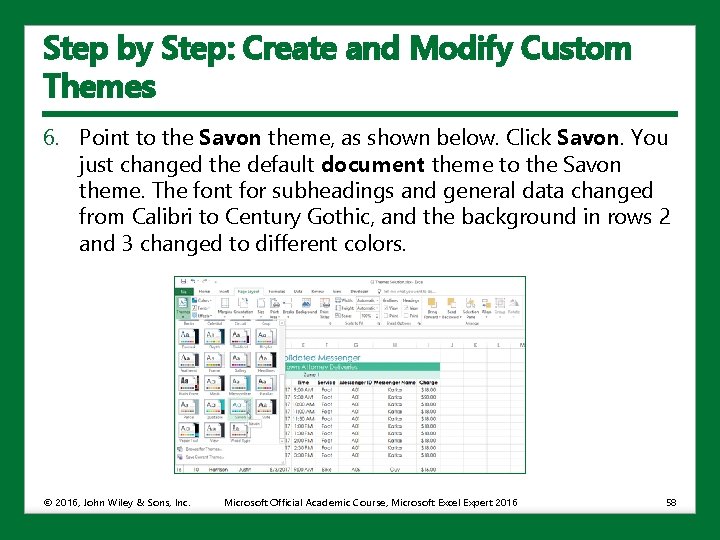
Step by Step: Create and Modify Custom Themes 6. Point to the Savon theme, as shown below. Click Savon. You just changed the default document theme to the Savon theme. The font for subheadings and general data changed from Calibri to Century Gothic, and the background in rows 2 and 3 changed to different colors. © 2016, John Wiley & Sons, Inc. Microsoft Official Academic Course, Microsoft Excel Expert 2016 58

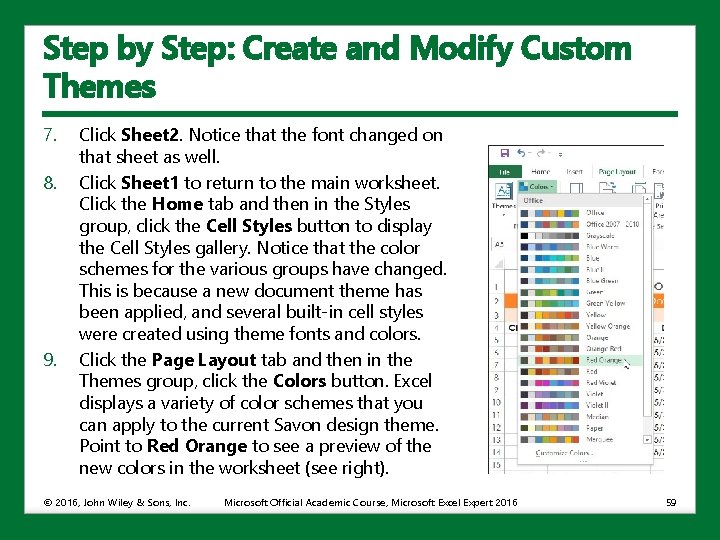
Step by Step: Create and Modify Custom Themes 7. 8. 9. Click Sheet 2. Notice that the font changed on that sheet as well. Click Sheet 1 to return to the main worksheet. Click the Home tab and then in the Styles group, click the Cell Styles button to display the Cell Styles gallery. Notice that the color schemes for the various groups have changed. This is because a new document theme has been applied, and several built-in cell styles were created using theme fonts and colors. Click the Page Layout tab and then in the Themes group, click the Colors button. Excel displays a variety of color schemes that you can apply to the current Savon design theme. Point to Red Orange to see a preview of the new colors in the worksheet (see right). © 2016, John Wiley & Sons, Inc. Microsoft Official Academic Course, Microsoft Excel Expert 2016 59

Step by Step: Create and Modify Custom Themes 10. From the Colors menu, click the Red Orange option. The fill colors in rows 2 and 3 have changed, but the fonts on both worksheets remain the same. 11. SAVE the workbook and CLOSE it. • LEAVE Excel open to use in the next exercise. • The default document theme in Excel 2016 is named Office. • Applying a new theme changes fonts and colors, and the color of shapes and Smart. Art, tables, charts, and other objects. • Remember that cell styles are used to format specific cells or ranges within a worksheet; document themes are used to apply sets of styles (colors, fonts, and fill effects) to an entire document. • Many built-in cell styles use theme-aware formatting, so applying a new theme determines which fonts and colors are used by styles. • That’s why you noticed a change in the Cell Styles gallery. • Styles are independent from themes in that you can change styles regardless of theme that’s applied. © 2016, John Wiley & Sons, Inc. Microsoft Official Academic Course, Microsoft Excel Expert 2016 60

Applying Custom Color Formats • In the previous exercise, you used the Colors button on the Page Layout tab to apply a different color scheme to the workbook. • Each color scheme includes individual colors for different worksheet elements that can be modified separately using the Create New Theme Colors dialog box. • This enables you to create custom color formats as needed in your worksheets. © 2016, John Wiley & Sons, Inc. Microsoft Official Academic Course, Microsoft Excel Expert 2016 61

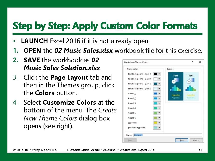
Step by Step: Apply Custom Color Formats • LAUNCH Excel 2016 if it is not already open. 1. OPEN the 02 Music Sales. xlsx workbook file for this exercise. 2. SAVE the workbook as 02 Music Sales Solution. xlsx. 3. Click the Page Layout tab and then in the Themes group, click the Colors button. 4. Select Customize Colors at the bottom of the menu. The Create New Theme Colors dialog box opens (see right). © 2016, John Wiley & Sons, Inc. Microsoft Official Academic Course, Microsoft Excel Expert 2016 62

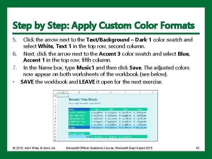
Step by Step: Apply Custom Color Formats 5. Click the arrow next to the Text/Background – Dark 1 color swatch and select White, Text 1 in the top row, second column. 6. Next, click the arrow next to the Accent 3 color swatch and select Blue, Accent 1 in the top row, fifth column. 7. In the Name box, type Music 1 and then click Save. The adjusted colors now appear on both worksheets of the workbook (see below). • SAVE the workbook and LEAVE it open for the next exercise. © 2016, John Wiley & Sons, Inc. Microsoft Official Academic Course, Microsoft Excel Expert 2016 63

Creating Custom Font Formats • You can customize the font themes used in a workbook. Excel provides dozens of font set choices, each consisting of a Heading font and a Body font, which you can modify as needed for a custom look. • You can choose new theme fonts in your worksheets using the Create New Theme Fonts dialog box. © 2016, John Wiley & Sons, Inc. Microsoft Official Academic Course, Microsoft Excel Expert 2016 64

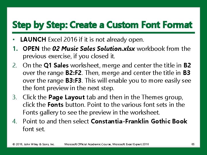
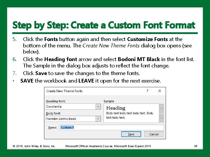
Step by Step: Create a Custom Font Format • LAUNCH Excel 2016 if it is not already open. 1. OPEN the 02 Music Sales Solution. xlsx workbook from the previous exercise, if you closed it. 2. On the Q 1 Sales worksheet, merge and center the title in B 2 over the range B 2: F 2. Then, merge and center the title in B 3 over the range B 3: F 3. This will enable you to more easily see the font preview in the next step. 3. Click the Page Layout tab and then in the Themes group, click the Fonts button. Point to the various font sets in the Fonts gallery to see the preview in the worksheet. 4. Point to and then select Constantia-Franklin Gothic Book font set. © 2016, John Wiley & Sons, Inc. Microsoft Official Academic Course, Microsoft Excel Expert 2016 65

Step by Step: Create a Custom Font Format 5. Click the Fonts button again and then select Customize Fonts at the bottom of the menu. The Create New Theme Fonts dialog box opens (see below). 6. Click the Heading font arrow and select Bodoni MT Black in the font list. The Sample in the dialog box adjusts to reflect the font change. 7. Click Save to save the changes to theme fonts. • SAVE the workbook and LEAVE it open for the next exercise. © 2016, John Wiley & Sons, Inc. Microsoft Official Academic Course, Microsoft Excel Expert 2016 66

Creating and Modifying Cell Styles • Excel provides many cell styles on the Cell Styles gallery of the Home tab that make it easy to apply fonts, fill colors, font styles, and borders with one click. • If none of the available options fit your needs, you can create a new cell style that can be applied at any time in any workbook. © 2016, John Wiley & Sons, Inc. Microsoft Official Academic Course, Microsoft Excel Expert 2016 67

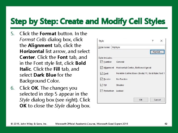
Step by Step: Create and Modify Cell Styles • LAUNCH Excel 2016 if it is not already open. 1. OPEN the 02 Music Sales Solution. xlsx workbook from the previous exercise, if you closed it. 2. On the Q 1 Sales worksheet, click cell B 5. You will start with the formatting that is already applied to this cell, make some changes, and then create a custom cell style. 3. On the Home tab, in the Styles group, click the Cell Styles button and then click New Cell Style at the bottom of the gallery. The New Cell Styles dialog box opens. 4. In the Style name box, type My. Style. Notice the existing styles applied to the style in the Style Includes (By Example) list in the dialog box. You can select or deselect check boxes to apply or remove any of these settings. © 2016, John Wiley & Sons, Inc. Microsoft Official Academic Course, Microsoft Excel Expert 2016 68

Step by Step: Create and Modify Cell Styles 5. 6. Click the Format button. In the Format Cells dialog box, click the Alignment tab, click the Horizontal list arrow, and select Center. Click the Font tab, and in the Font style list, click Bold Italic. Click the Fill tab, and select Dark Blue for the Background Color. Click OK. The changes you selected in step 5 appear in the Style dialog box (see right). Click OK to close the Style dialog box. © 2016, John Wiley & Sons, Inc. Microsoft Official Academic Course, Microsoft Excel Expert 2016 69

Step by Step: Create and Modify Cell Styles 7. With B 5 selected, click the Cell Styles button on the Home tab, and select My. Style at the top of the gallery. Your new style is applied to cell B 5. 8. After applying the cell style, you decide to remove the italic formatting from the custom style. Click the Cell Styles button on the Home tab, right-click My. Style at the top of the gallery, and select Modify. The Style dialog box opens. 9. Click the Format button. In the Format Cells dialog box, click the Font tab if necessary, and in the Font style list, click Bold. 10. Click OK two times to close both dialog boxes. Cell B 5 now displays the modified style without italics. 11. SAVE the workbook and CLOSE it. • LEAVE Excel open to use in the next exercise. © 2016, John Wiley & Sons, Inc. Microsoft Official Academic Course, Microsoft Excel Expert 2016 70

Recording and Modifying a Basic Macro • A basic macro is a recording of a sequence of commands and typed entries that you can then replay elsewhere in the worksheet. • Macros enable you to perform the same sequences of commands in different places, cutting down the time it takes to complete redundant work. • There are ways to automate the formatting of cells that are actually easier than recording and playing back macros. • So the types of steps you want to record are the repetitious kind that you would otherwise have to repeat yourself dozens of times or more. © 2016, John Wiley & Sons, Inc. Microsoft Official Academic Course, Microsoft Excel Expert 2016 71

Step by Step: Record and Modify a Basic Macro • LAUNCH Excel 2016 if it is not already open. 1. OPEN the 02 Revenues. xlsx workbook file for this exercise. If the Developer tab is already displayed on the ribbon, skip to step 5. 2. Click the File tab and then click Options. 3. In the Excel Options dialog box, click Customize Ribbon. 4. In the Main Tabs list on the right, select the Developer check box. This adds the Developer tab to the Excel ribbon, enabling you to more easily record macros. Click OK. 5. The macro that you record creates a custom subtotal row at the place you define, rather than at some place Excel determines. The rule you follow is that the user (you) must select the cell where you want the subtotal to appear, and then run the macro. So to prepare for macro recording, click cell D 20. © 2016, John Wiley & Sons, Inc. Microsoft Official Academic Course, Microsoft Excel Expert 2016 72

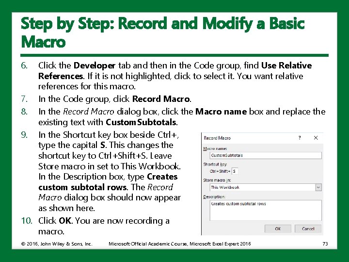
Step by Step: Record and Modify a Basic Macro 6. Click the Developer tab and then in the Code group, find Use Relative References. If it is not highlighted, click to select it. You want relative references for this macro. 7. In the Code group, click Record Macro. 8. In the Record Macro dialog box, click the Macro name box and replace the existing text with Custom. Subtotals. 9. In the Shortcut key box beside Ctrl+, type the capital S. This changes the shortcut key to Ctrl+Shift+S. Leave Store macro in set to This Workbook. In the Description box, type Creates custom subtotal rows. The Record Macro dialog box should now appear as shown here. 10. Click OK. You are now recording a macro. © 2016, John Wiley & Sons, Inc. Microsoft Official Academic Course, Microsoft Excel Expert 2016 73

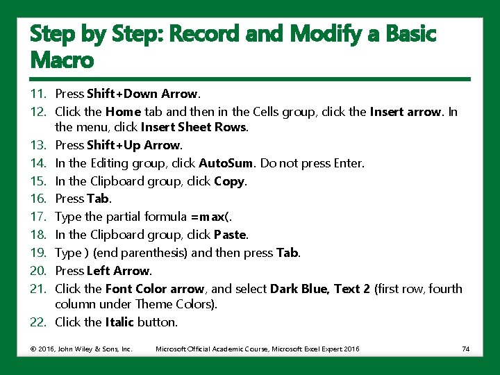
Step by Step: Record and Modify a Basic Macro 11. Press Shift+Down Arrow. 12. Click the Home tab and then in the Cells group, click the Insert arrow. In the menu, click Insert Sheet Rows. 13. Press Shift+Up Arrow. 14. In the Editing group, click Auto. Sum. Do not press Enter. 15. In the Clipboard group, click Copy. 16. Press Tab. 17. Type the partial formula =max(. 18. In the Clipboard group, click Paste. 19. Type ) (end parenthesis) and then press Tab. 20. Press Left Arrow. 21. Click the Font Color arrow, and select Dark Blue, Text 2 (first row, fourth column under Theme Colors). 22. Click the Italic button. © 2016, John Wiley & Sons, Inc. Microsoft Official Academic Course, Microsoft Excel Expert 2016 74

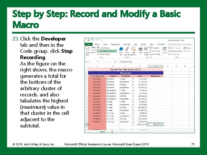
Step by Step: Record and Modify a Basic Macro 23. Click the Developer tab and then in the Code group, click Stop Recording. As the figure on the right shows, the macro generates a total for the bottom of the arbitrary cluster of records, and also tabulates the highest (maximum) value in that cluster in the cell adjacent to the subtotal. © 2016, John Wiley & Sons, Inc. Microsoft Official Academic Course, Microsoft Excel Expert 2016 75

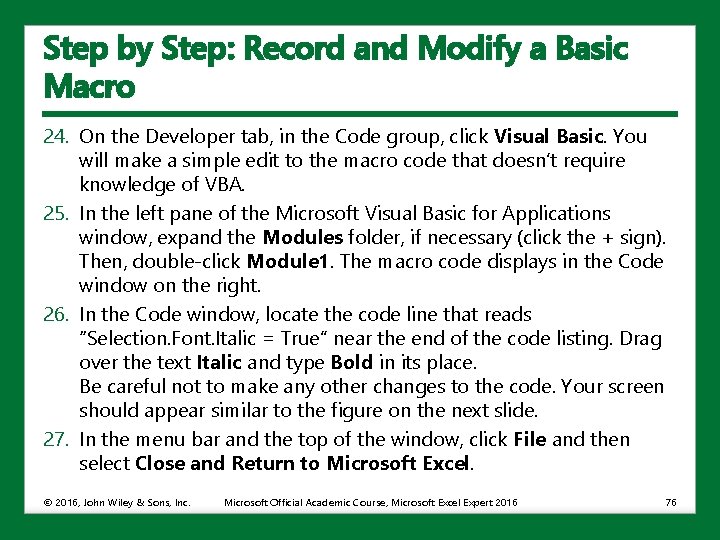
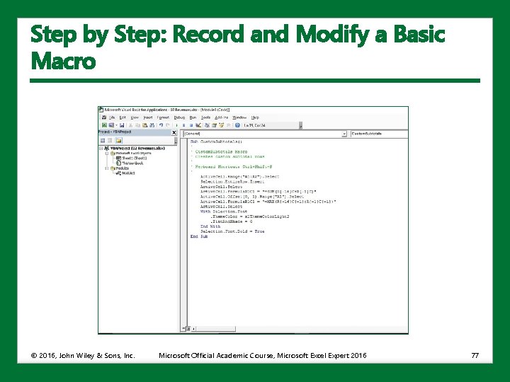
Step by Step: Record and Modify a Basic Macro 24. On the Developer tab, in the Code group, click Visual Basic. You will make a simple edit to the macro code that doesn’t require knowledge of VBA. 25. In the left pane of the Microsoft Visual Basic for Applications window, expand the Modules folder, if necessary (click the + sign). Then, double-click Module 1. The macro code displays in the Code window on the right. 26. In the Code window, locate the code line that reads “Selection. Font. Italic = True” near the end of the code listing. Drag over the text Italic and type Bold in its place. Be careful not to make any other changes to the code. Your screen should appear similar to the figure on the next slide. 27. In the menu bar and the top of the window, click File and then select Close and Return to Microsoft Excel. © 2016, John Wiley & Sons, Inc. Microsoft Official Academic Course, Microsoft Excel Expert 2016 76

Step by Step: Record and Modify a Basic Macro © 2016, John Wiley & Sons, Inc. Microsoft Official Academic Course, Microsoft Excel Expert 2016 77

Managing Macro Security • Because of the proliferation of malicious software, Microsoft has set up Excel so that after it’s installed, you cannot execute macros from a file you open (even an explicitly macro-enabled workbook) until you read the notification and click Enable Content. • If you never plan to run macros or if you’re skeptical about your office colleagues, you can turn off macros completely. • You can also turn off the notifications and enable all macros, if you work in an office such as a financial services provider where macros are in use constantly, you trust the source of the Excel workbooks, and notifications would only get in the way. © 2016, John Wiley & Sons, Inc. Microsoft Official Academic Course, Microsoft Excel Expert 2016 78

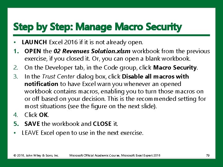
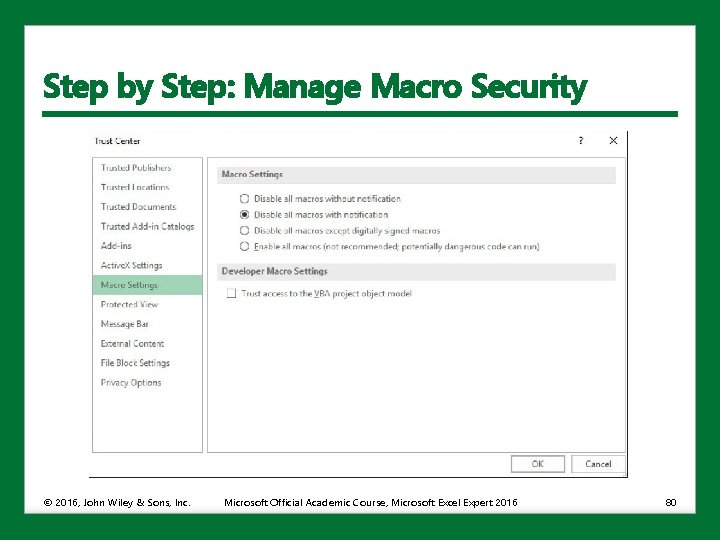
Step by Step: Manage Macro Security • LAUNCH Excel 2016 if it is not already open. 1. OPEN the 02 Revenues Solution. xlsm workbook from the previous exercise, if you closed it. Or, you can open a blank workbook. 2. On the Developer tab, in the Code group, click Macro Security. 3. In the Trust Center dialog box, click Disable all macros with notification to have Excel warn you whenever an opened workbook contains macros, enabling you to turn those macros on or off based on your decision. This is the recommended setting for most situations (see the figure on the next slide). 4. Click OK. 5. SAVE the workbook and CLOSE it. • LEAVE Excel open to use in the next exercise. © 2016, John Wiley & Sons, Inc. Microsoft Official Academic Course, Microsoft Excel Expert 2016 79

Step by Step: Manage Macro Security © 2016, John Wiley & Sons, Inc. Microsoft Official Academic Course, Microsoft Excel Expert 2016 80

Inserting Form Controls • If you are developing a workbook that other people are going to use, your users might find it helpful if you add controls such as check boxes, command buttons, and spin buttons. • Adding controls to a workbook helps limit a user’s choices or to make the available choices easier to select. • Excel offers two families of controls: • Form controls: Native to Excel and are backward compatible to Excel 95. • Active. X controls: Used in a variety of applications besides Excel, and can be controlled via VBA. You can add VBA to your workbook to respond to events. Active. X controls also have more options or properties you can control. © 2016, John Wiley & Sons, Inc. Microsoft Official Academic Course, Microsoft Excel Expert 2016 81

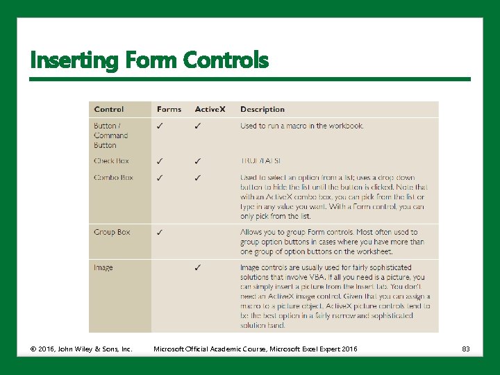
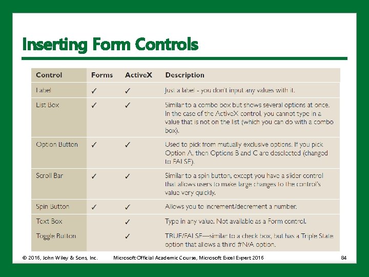
Inserting Form Controls • Both types of controls offer the ability to link input (populate a list) and output (show what was selected) between the control and a worksheet cell. • Note that both Form controls and Active. X controls float on the worksheet. • This means that like shapes, you can tell Excel whether you want to move and/or resize your controls as you insert, delete, or resize rows and columns. • A basic listing of the available form controls includes the ones shown in the table on the following slides. © 2016, John Wiley & Sons, Inc. Microsoft Official Academic Course, Microsoft Excel Expert 2016 82

Inserting Form Controls © 2016, John Wiley & Sons, Inc. Microsoft Official Academic Course, Microsoft Excel Expert 2016 83

Inserting Form Controls © 2016, John Wiley & Sons, Inc. Microsoft Official Academic Course, Microsoft Excel Expert 2016 84

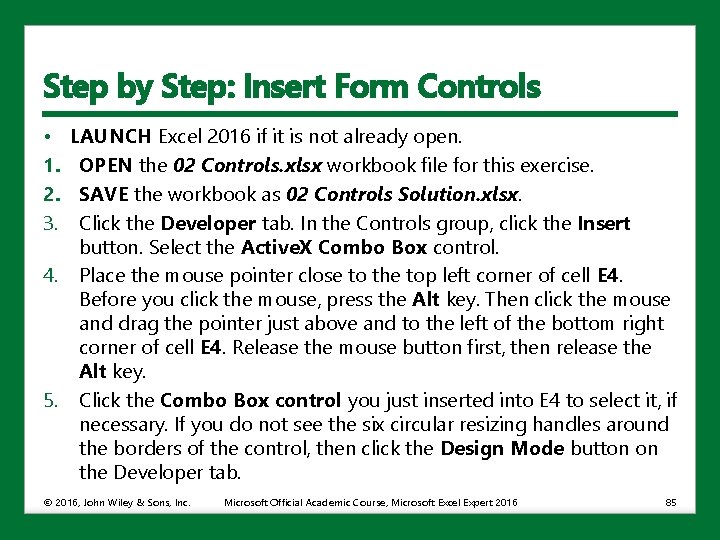
Step by Step: Insert Form Controls • 1. 2. 3. LAUNCH Excel 2016 if it is not already open. OPEN the 02 Controls. xlsx workbook file for this exercise. SAVE the workbook as 02 Controls Solution. xlsx. Click the Developer tab. In the Controls group, click the Insert button. Select the Active. X Combo Box control. 4. Place the mouse pointer close to the top left corner of cell E 4. Before you click the mouse, press the Alt key. Then click the mouse and drag the pointer just above and to the left of the bottom right corner of cell E 4. Release the mouse button first, then release the Alt key. 5. Click the Combo Box control you just inserted into E 4 to select it, if necessary. If you do not see the six circular resizing handles around the borders of the control, then click the Design Mode button on the Developer tab. © 2016, John Wiley & Sons, Inc. Microsoft Official Academic Course, Microsoft Excel Expert 2016 85

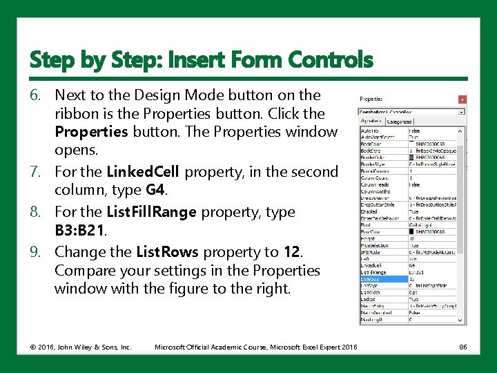
Step by Step: Insert Form Controls 6. Next to the Design Mode button on the ribbon is the Properties button. Click the Properties button. The Properties window opens. 7. For the Linked. Cell property, in the second column, type G 4. 8. For the List. Fill. Range property, type B 3: B 21. 9. Change the List. Rows property to 12. Compare your settings in the Properties window with the figure to the right. © 2016, John Wiley & Sons, Inc. Microsoft Official Academic Course, Microsoft Excel Expert 2016 86

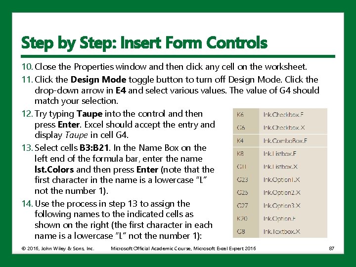
Step by Step: Insert Form Controls 10. Close the Properties window and then click any cell on the worksheet. 11. Click the Design Mode toggle button to turn off Design Mode. Click the drop-down arrow in E 4 and select various values. The value of G 4 should match your selection. 12. Try typing Taupe into the control and then press Enter. Excel should accept the entry and display Taupe in cell G 4. 13. Select cells B 3: B 21. In the Name Box on the left end of the formula bar, enter the name lst. Colors and then press Enter (note that the first character in the name is a lowercase “L” not the number 1). 14. Use the process in step 13 to assign the following names to the indicated cells as shown on the right (the first character in each name is a lowercase “L” not the number 1): © 2016, John Wiley & Sons, Inc. Microsoft Official Academic Course, Microsoft Excel Expert 2016 87

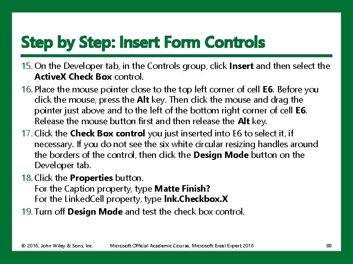
Step by Step: Insert Form Controls 15. On the Developer tab, in the Controls group, click Insert and then select the Active. X Check Box control. 16. Place the mouse pointer close to the top left corner of cell E 6. Before you click the mouse, press the Alt key. Then click the mouse and drag the pointer just above and to the left of the bottom right corner of cell E 6. Release the mouse button first and then release the Alt key. 17. Click the Check Box control you just inserted into E 6 to select it, if necessary. If you do not see the six white circular resizing handles around the borders of the control, then click the Design Mode button on the Developer tab. 18. Click the Properties button. For the Caption property, type Matte Finish? For the Linked. Cell property, type lnk. Checkbox. X 19. Turn off Design Mode and test the check box control. © 2016, John Wiley & Sons, Inc. Microsoft Official Academic Course, Microsoft Excel Expert 2016 88

Step by Step: Insert Form Controls 20. Repeat previous instructions as appropriate to add the following controls: An Active. X Text Box control in E 8 with a Linked. Cell property of lnk. Textbox. X An Active. X List Box control in E 11: E 21, Linked. Cell property is lnk. Listbox. X and the List. Fill. Range is lst. Colors An Active. X Option Button control in E 23, Linked. Cell property is lnk. Option 1. X and the Caption is Matte Finish An Active. X Option Button control in E 25, Linked. Cell property is lnk. Option 2. X and the Caption is Glossy Finish An Active. X Option Button control in E 27, Linked. Cell property is lnk. Option 3. X and the Caption is No Finish 21. Close the Properties window, turn off Design Mode, and test your controls. © 2016, John Wiley & Sons, Inc. Microsoft Official Academic Course, Microsoft Excel Expert 2016 89

Step by Step: Insert Form Controls 22. On the Developer tab, click the Insert button. This time insert a Form control Combo Box into cell I 4. 23. Right-click the combo box control and select Format Control from the shortcut menu. Select the Control tab. 24. Set the Input range to lst. Colors and the Cell link to lnk. Combo. Box. F and then click OK. 25. Click any regular cell. If the pointer changes into a pointing finger when you mouse over the control in cell I 4, then you can use it. 26. Try typing Taupe into the Forms combo box in cell I 4. Unlike the Active. X combo box, you can’t type into a Forms combo box. 27. Place a Form control check box in I 6. 28. Right-click the check box and select Format Control. 29. On the Control tab, set the Cell link to lnk. Checkbox. F. © 2016, John Wiley & Sons, Inc. Microsoft Official Academic Course, Microsoft Excel Expert 2016 90

Step by Step: Insert Form Controls 30. Click the Alt Text tab and change the alternative text to Matte Finish? Click OK. 31. Click in cell H 6 then press the right-arrow key once. Then press Delete. This will clear out the text in I 6 so you can read the check box better. 32. Notice that changing the Alt Text in step 30 didn’t change the check box’s caption. Right-click the check box control and select Edit Text to change the caption to Matte Finish? . 33. Place a Form control list box across cells I 8: I 18. (Remember, if you press the Alt key prior to starting your drag, the control will snap to the cell borders. ) 34. Right-click the list box and select Format Control from the shortcut menu. Make the following entries: Input range = lst. Colors Cell link = lnk. Listbox. F © 2016, John Wiley & Sons, Inc. Microsoft Official Academic Course, Microsoft Excel Expert 2016 91

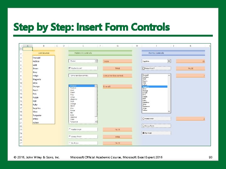
Step by Step: Insert Form Controls 35. Click OK and then select any cell in the worksheet. Test your Forms list box control. 36. Delete the text in cells I 20, I 22 and I 24 37. Place a Form control Option Button in cell I 20 and edit the text to read Matte Finish. 38. Place a Form control Option Button in cell I 22 and edit the text to read Glossy Finish. 39. Place a Form control Option Button in cell I 24 and edit the text to read No Finish. 40. Right-click any of the Option Button controls and select Format Control. Click the Control tab, set the Cell link to lnk. Option. F, and then click OK. Your worksheet should now look similar to the figure on the next slide. © 2016, John Wiley & Sons, Inc. Microsoft Official Academic Course, Microsoft Excel Expert 2016 92

Step by Step: Insert Form Controls © 2016, John Wiley & Sons, Inc. Microsoft Official Academic Course, Microsoft Excel Expert 2016 93

Step by Step: Insert Form Controls 41. Play with the controls a bit and notice that the Active. X combo box and list box controls are returning the text you select. Compare this to the Form combo box and list box. Both of those return the index (position) of your choice in the list of choices. 42. SAVE the workbook and CLOSE it. • LEAVE Excel open to use in the next exercise. • Note that in the case of option button controls, all three Form control option buttons have the same linked cell and this linked cell contains the index of whichever option button is selected. • Compare that to the Active. X option buttons where each option button has its own linked cell and each linked cell toggles between TRUE and FALSE. © 2016, John Wiley & Sons, Inc. Microsoft Official Academic Course, Microsoft Excel Expert 2016 94

Preparing a Workbook for Internationalization • • In today’s global economy, you may find yourself frequently exchanging workbooks with overseas affiliates. If you need to enter text and perform a spell check in a foreign language, click the File tab, click Options, and then select Language in the left pane. Here, you can additional language dictionaries for spell checks and proofing. Click the drop-down arrow to add a proofing dictionary. If that dictionary does not come pre-installed for your part of the world, you will see a Proofing status of “Not installed. ” You’ll need to click that status (it’s a hyperlink) and then locate and download the dictionary you seek. The Language section of the Excel Options dialog box is also where you can alter the language in which Excel is displayed, the language for Help information, and the language for Screen. Tips. © 2016, John Wiley & Sons, Inc. Microsoft Official Academic Course, Microsoft Excel Expert 2016 95

Step by Step: Apply International Symbols and Currency • 1. 2. 3. LAUNCH Excel 2016 if it is not already open. OPEN the 02 International. xlsx workbook file for this exercise. SAVE the workbook as 02 International Solution. xlsx. Click cell C 7, press F 2, and then press Home to enter edit mode and position the cursor at the beginning of the cell’s text. 4. Press the right arrow key twice to position the cursor directly after the first “a” and then press the Backspace key to delete the “a”. 5. Click the Insert tab. On the right end of the tab, notice that the Symbol button is still enabled while in edit mode. Click the Symbol button. The Symbol dialog box opens. 6. In the Font box at the top-left corner of the dialog box, the Font should be Calibri. If it is anything other than Calibri, change it to Calibri. © 2016, John Wiley & Sons, Inc. Microsoft Official Academic Course, Microsoft Excel Expert 2016 96

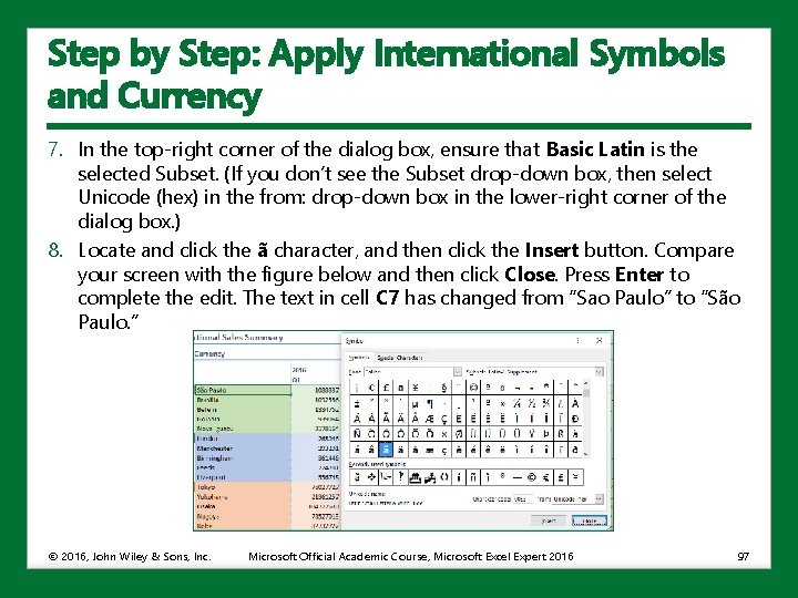
Step by Step: Apply International Symbols and Currency 7. In the top-right corner of the dialog box, ensure that Basic Latin is the selected Subset. (If you don’t see the Subset drop-down box, then select Unicode (hex) in the from: drop-down box in the lower-right corner of the dialog box. ) 8. Locate and click the ã character, and then click the Insert button. Compare your screen with the figure below and then click Close. Press Enter to complete the edit. The text in cell C 7 has changed from “Sao Paulo” to “São Paulo. ” © 2016, John Wiley & Sons, Inc. Microsoft Official Academic Course, Microsoft Excel Expert 2016 97

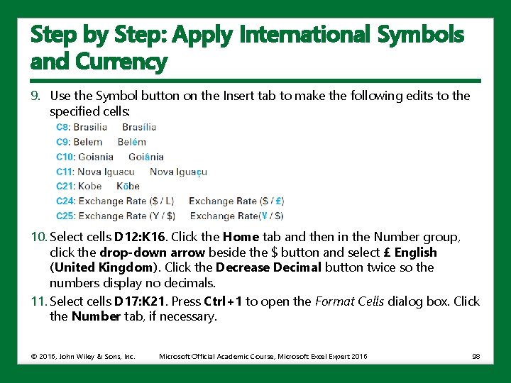
Step by Step: Apply International Symbols and Currency 9. Use the Symbol button on the Insert tab to make the following edits to the specified cells: 10. Select cells D 12: K 16. Click the Home tab and then in the Number group, click the drop-down arrow beside the $ button and select £ English (United Kingdom). Click the Decrease Decimal button twice so the numbers display no decimals. 11. Select cells D 17: K 21. Press Ctrl+1 to open the Format Cells dialog box. Click the Number tab, if necessary. © 2016, John Wiley & Sons, Inc. Microsoft Official Academic Course, Microsoft Excel Expert 2016 98

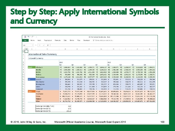
Step by Step: Apply International Symbols and Currency 12. In the Category list, select Accounting. Change the Decimal places to 0. In the Symbol drop-down list, select ¥ Japanese (unfortunately, the Symbol list is not sorted alphabetically so you just have to scroll until you find it). Click OK. 13. Select D 7: K 11 and then press Ctrl+1 again. 14. Set the number format to Accounting with 0 Decimal places. Leave the Symbol as a dollar sign. 15. In the Category list, change the category to Custom and then edit the number format, placing a backslash and an R in front of each $ symbol so that it reads: _(R$* #, ##0_); _(R$* (#, ##0); _(R$* “-”_); _(@_) 16. Click OK. Press Ctrl+Home and then compare your worksheet with the figure on the next slide. 17. SAVE the workbook and CLOSE it. • CLOSE Excel. © 2016, John Wiley & Sons, Inc. Microsoft Official Academic Course, Microsoft Excel Expert 2016 99

Step by Step: Apply International Symbols and Currency © 2016, John Wiley & Sons, Inc. Microsoft Official Academic Course, Microsoft Excel Expert 2016 100

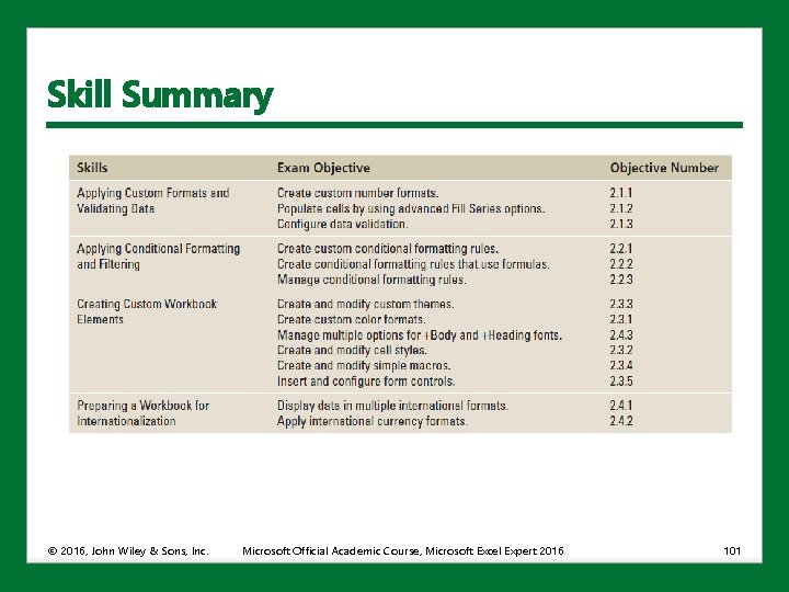
Skill Summary © 2016, John Wiley & Sons, Inc. Microsoft Official Academic Course, Microsoft Excel Expert 2016 101