Microsoft Excel 2016 Lesson 8 Managing Worksheets 2016

Microsoft Excel 2016 Lesson 8 Managing Worksheets © 2016, John Wiley & Sons, Inc. Microsoft Official Academic Course, Microsoft Excel Core 2016 1

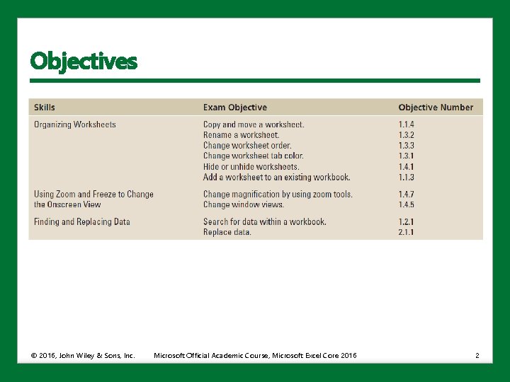
Objectives © 2016, John Wiley & Sons, Inc. Microsoft Official Academic Course, Microsoft Excel Core 2016 2

Software Orientation • Think of an Excel workbook as a collection of the types of things you have previously recorded on paper and stored in a folder that was then filed in a cabinet. • A workbook does not have to include the contents of the entire cabinet, just the records that pertain to one subject. • Business transactions that take place during a period of time, such as a specific week or month, might make up a workbook. • You can divide a workbook into sheets to subcategorize transactions into days. • Another option is to have each sheet represent a certain sales department. • In this lesson, you become familiar with how you can manipulate worksheets within a workbook. © 2016, John Wiley & Sons, Inc. Microsoft Official Academic Course, Microsoft Excel Core 2016 3

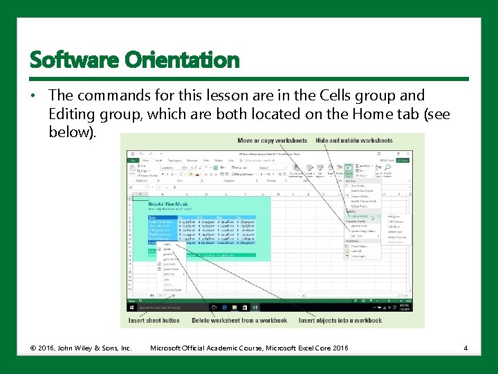
Software Orientation • The commands for this lesson are in the Cells group and Editing group, which are both located on the Home tab (see below). © 2016, John Wiley & Sons, Inc. Microsoft Official Academic Course, Microsoft Excel Core 2016 4

Organizing Worksheets • A new Excel workbook has one blank worksheet by default. • There’s no practical limit to how many worksheets a workbook can contain. • The order of worksheets in a workbook is determined by the sequence of tabs along the bottom of the Excel window. • You use these tabs to switch between worksheets in the window. • You can arrange worksheets in a sensible order that helps you find them easier and keep related content grouped. © 2016, John Wiley & Sons, Inc. Microsoft Official Academic Course, Microsoft Excel Core 2016 5

Copying a Worksheet • There’s a clear difference between copying the contents of a worksheet into another worksheet and copying worksheets in their entirety. • One big reason you’d want to copy worksheets entirely is to create a new worksheet that’s identical in style and format to an existing one to enter new data. • Copying a worksheet duplicates everything, including formatting, data, and formulas. © 2016, John Wiley & Sons, Inc. Microsoft Official Academic Course, Microsoft Excel Core 2016 6

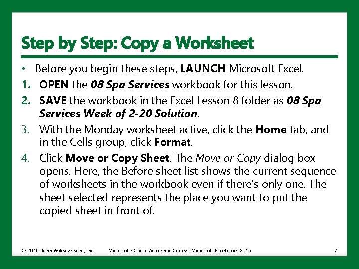
Step by Step: Copy a Worksheet • Before you begin these steps, LAUNCH Microsoft Excel. 1. OPEN the 08 Spa Services workbook for this lesson. 2. SAVE the workbook in the Excel Lesson 8 folder as 08 Spa Services Week of 2 -20 Solution. 3. With the Monday worksheet active, click the Home tab, and in the Cells group, click Format. 4. Click Move or Copy Sheet. The Move or Copy dialog box opens. Here, the Before sheet list shows the current sequence of worksheets in the workbook even if there’s only one. The sheet selected represents the place you want to put the copied sheet in front of. © 2016, John Wiley & Sons, Inc. Microsoft Official Academic Course, Microsoft Excel Core 2016 7

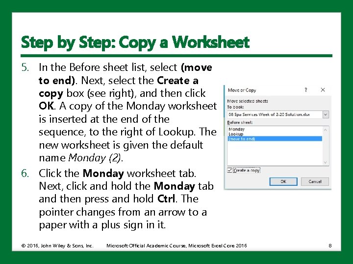
Step by Step: Copy a Worksheet 5. In the Before sheet list, select (move to end). Next, select the Create a copy box (see right), and then click OK. A copy of the Monday worksheet is inserted at the end of the sequence, to the right of Lookup. The new worksheet is given the default name Monday (2). 6. Click the Monday worksheet tab. Next, click and hold the Monday tab and then press and hold Ctrl. The pointer changes from an arrow to a paper with a plus sign in it. © 2016, John Wiley & Sons, Inc. Microsoft Official Academic Course, Microsoft Excel Core 2016 8

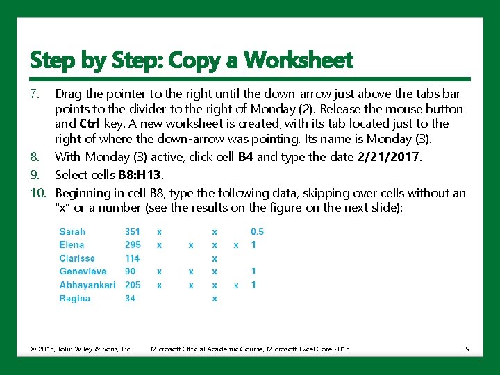
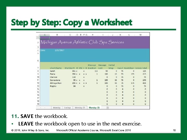
Step by Step: Copy a Worksheet 7. Drag the pointer to the right until the down-arrow just above the tabs bar points to the divider to the right of Monday (2). Release the mouse button and Ctrl key. A new worksheet is created, with its tab located just to the right of where the down-arrow was pointing. Its name is Monday (3). 8. With Monday (3) active, click cell B 4 and type the date 2/21/2017. 9. Select cells B 8: H 13. 10. Beginning in cell B 8, type the following data, skipping over cells without an “x” or a number (see the results on the figure on the next slide): © 2016, John Wiley & Sons, Inc. Microsoft Official Academic Course, Microsoft Excel Core 2016 9

Step by Step: Copy a Worksheet 11. SAVE the workbook. • LEAVE the workbook open to use in the next exercise. © 2016, John Wiley & Sons, Inc. Microsoft Official Academic Course, Microsoft Excel Core 2016 10

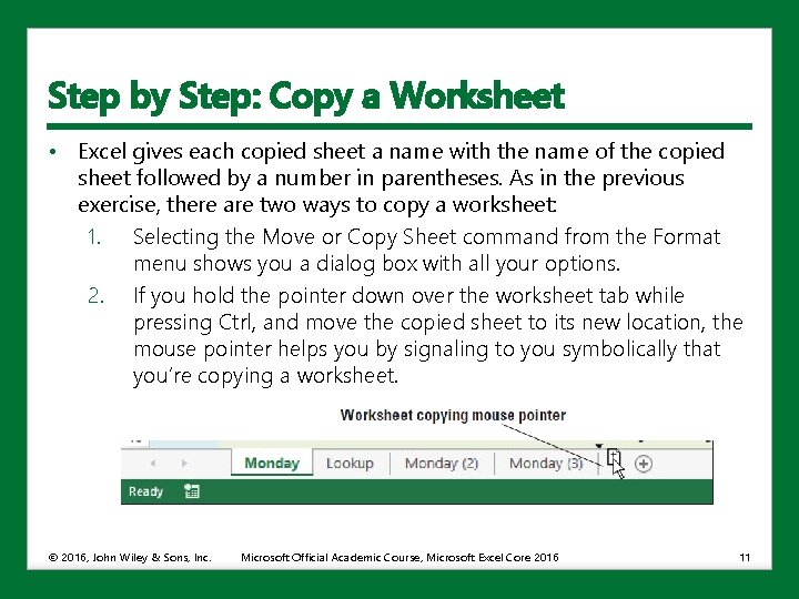
Step by Step: Copy a Worksheet • Excel gives each copied sheet a name with the name of the copied sheet followed by a number in parentheses. As in the previous exercise, there are two ways to copy a worksheet: 1. Selecting the Move or Copy Sheet command from the Format menu shows you a dialog box with all your options. 2. If you hold the pointer down over the worksheet tab while pressing Ctrl, and move the copied sheet to its new location, the mouse pointer helps you by signaling to you symbolically that you’re copying a worksheet. © 2016, John Wiley & Sons, Inc. Microsoft Official Academic Course, Microsoft Excel Core 2016 11

Renaming a Worksheet • Excel gives a newly inserted or copied worksheet a temporary name, such as Sheet 2, Sheet 3, or Monday (2), as in the example. • In the example, obviously we don’t want multiple Mondays, and the day for which you just entered transactions happens to be Tuesday. © 2016, John Wiley & Sons, Inc. Microsoft Official Academic Course, Microsoft Excel Core 2016 12

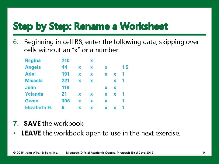
Step by Step: Rename a Worksheet • USE the workbook from the previous exercise. 1. Double-click the Monday (3) worksheet tab to select its name. 2. Type Tuesday and then press Enter. The new name appears on the tab. 3. Repeat this process for the Monday (2) worksheet tab, renaming it Wednesday. 4. With the Wednesday worksheet active, select cell B 4 and type the date 2/22/2017. 5. Select cells B 8: H 15. © 2016, John Wiley & Sons, Inc. Microsoft Official Academic Course, Microsoft Excel Core 2016 13

Step by Step: Rename a Worksheet 6. Beginning in cell B 8, enter the following data, skipping over cells without an “x” or a number. 7. SAVE the workbook. • LEAVE the workbook open to use in the next exercise. © 2016, John Wiley & Sons, Inc. Microsoft Official Academic Course, Microsoft Excel Core 2016 14

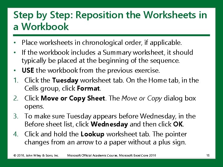
Step by Step: Reposition the Worksheets in a Workbook • Place worksheets in chronological order, if applicable. • If the workbook includes a Summary worksheet, it should typically be placed at the beginning of the sequence. • USE the workbook from the previous exercise. 1. Click the Tuesday worksheet tab. On the Home tab, in the Cells group, click Format. 2. Click Move or Copy Sheet. The Move or Copy dialog box opens. 3. To make sure Tuesday appears before Wednesday, in the Before sheet list, click Wednesday and then click OK. 4. Click and hold the Lookup worksheet tab. The pointer changes from an arrow to a paper without a plus sign. © 2016, John Wiley & Sons, Inc. Microsoft Official Academic Course, Microsoft Excel Core 2016 15

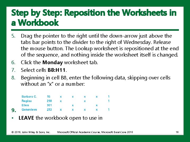
Step by Step: Reposition the Worksheets in a Workbook 5. 6. 7. 8. Drag the pointer to the right until the down-arrow just above the tabs bar points to the divider to the right of Wednesday. Release the mouse button. The Lookup worksheet is repositioned at the end of the sequence, and nothing inside the worksheet itself is changed. Click the Monday worksheet tab. Select cells B 8: H 11. Beginning in cell B 8, enter the following data, skipping over cells without an “x” or a number: 9. SAVE the workbook. • LEAVE the workbook open to use in © 2016, John Wiley & Sons, Inc. Microsoft Official Academic Course, Microsoft Excel Core 2016 16

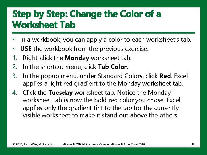
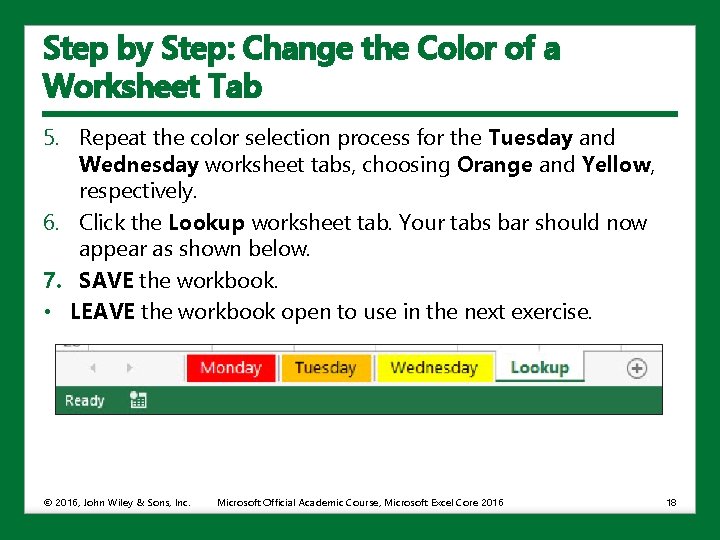
Step by Step: Change the Color of a Worksheet Tab • • 1. 2. 3. In a workbook, you can apply a color to each worksheet’s tab. USE the workbook from the previous exercise. Right-click the Monday worksheet tab. In the shortcut menu, click Tab Color. In the popup menu, under Standard Colors, click Red. Excel applies a light red gradient to the Monday worksheet tab. 4. Click the Tuesday worksheet tab. Notice the Monday worksheet tab is now the bold red color you chose. Excel applies only the gradient tint to the tab for the currently visible worksheet to make it stand out above the others. © 2016, John Wiley & Sons, Inc. Microsoft Official Academic Course, Microsoft Excel Core 2016 17

Step by Step: Change the Color of a Worksheet Tab 5. Repeat the color selection process for the Tuesday and Wednesday worksheet tabs, choosing Orange and Yellow, respectively. 6. Click the Lookup worksheet tab. Your tabs bar should now appear as shown below. 7. SAVE the workbook. • LEAVE the workbook open to use in the next exercise. © 2016, John Wiley & Sons, Inc. Microsoft Official Academic Course, Microsoft Excel Core 2016 18

Hiding and Unhiding Worksheets • Not every element of data in a workbook needs to be visible to every user, such as lookup tables and other auxiliary data. • This type of data might need to be updated from time to time, but it doesn’t need to display to everyone using the workbook. • You can hide a worksheet and unhide it to work with it again. • Hiding a worksheet does not make it confidential, because all worksheets are easy to unhide. • Hiding simply gets it out of your way. © 2016, John Wiley & Sons, Inc. Microsoft Official Academic Course, Microsoft Excel Core 2016 19

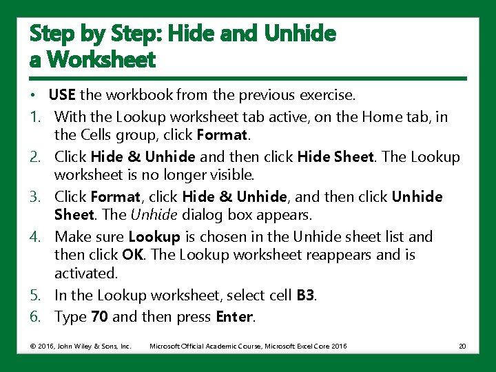
Step by Step: Hide and Unhide a Worksheet • USE the workbook from the previous exercise. 1. With the Lookup worksheet tab active, on the Home tab, in the Cells group, click Format. 2. Click Hide & Unhide and then click Hide Sheet. The Lookup worksheet is no longer visible. 3. Click Format, click Hide & Unhide, and then click Unhide Sheet. The Unhide dialog box appears. 4. Make sure Lookup is chosen in the Unhide sheet list and then click OK. The Lookup worksheet reappears and is activated. 5. In the Lookup worksheet, select cell B 3. 6. Type 70 and then press Enter. © 2016, John Wiley & Sons, Inc. Microsoft Official Academic Course, Microsoft Excel Core 2016 20

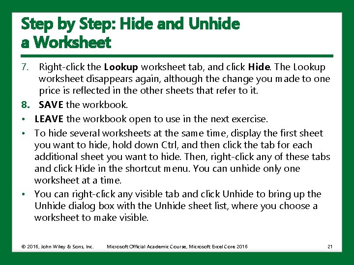
Step by Step: Hide and Unhide a Worksheet 7. 8. • • • Right-click the Lookup worksheet tab, and click Hide. The Lookup worksheet disappears again, although the change you made to one price is reflected in the other sheets that refer to it. SAVE the workbook. LEAVE the workbook open to use in the next exercise. To hide several worksheets at the same time, display the first sheet you want to hide, hold down Ctrl, and then click the tab for each additional sheet you want to hide. Then, right-click any of these tabs and click Hide in the shortcut menu. You can unhide only one worksheet at a time. You can right-click any visible tab and click Unhide to bring up the Unhide dialog box with the Unhide sheet list, where you choose a worksheet to make visible. © 2016, John Wiley & Sons, Inc. Microsoft Official Academic Course, Microsoft Excel Core 2016 21

Inserting a New Worksheet into a Workbook • In Excel 2016, a new workbook contains only one worksheet. • You should keep the number of worksheets down to a handful. • If your tasks are so complex that you need dozens of worksheets, consider dividing sheets among multiple workbooks. • Excel recognizes cell references that cross workbook boundaries, so your workbooks are not limited to worksheets that relate just to one another. © 2016, John Wiley & Sons, Inc. Microsoft Official Academic Course, Microsoft Excel Core 2016 22

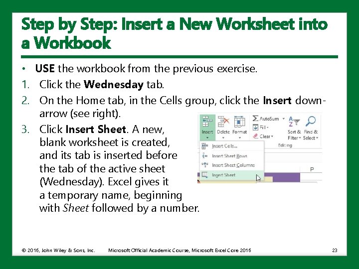
Step by Step: Insert a New Worksheet into a Workbook • USE the workbook from the previous exercise. 1. Click the Wednesday tab. 2. On the Home tab, in the Cells group, click the Insert downarrow (see right). 3. Click Insert Sheet. A new, blank worksheet is created, and its tab is inserted before the tab of the active sheet (Wednesday). Excel gives it a temporary name, beginning with Sheet followed by a number. © 2016, John Wiley & Sons, Inc. Microsoft Official Academic Course, Microsoft Excel Core 2016 23

Step by Step: Insert a New Worksheet into a Workbook 4. 5. 6. 7. Move the new worksheet to the end of the tab sequence. Rename the new worksheet Survey. Click the Wednesday worksheet tab again. Click the New Sheet (+) button to the right of the worksheet tabs. Another new worksheet is created with a temporary name, and this time, its tab is inserted after Wednesday. 8. Rename this new worksheet Totals. 9. SAVE the workbook. • LEAVE the workbook open to use in the next exercise. © 2016, John Wiley & Sons, Inc. Microsoft Official Academic Course, Microsoft Excel Core 2016 24

Step by Step: Delete a Worksheet from a Workbook • Be sure the contents of a worksheet you’re about to delete are not referred to or required by any element in another worksheet. • USE the workbook from the previous exercise. 1. Click the Totals worksheet tab. 2. On the Home tab, in the Cells group, click the Delete down-arrow. 3. Click Delete Sheet. The Totals worksheet is removed and its tab disappears. 4. Right-click the Survey tab, and click Delete. The Survey worksheet is removed and its tab disappears. 5. SAVE the workbook. • LEAVE the workbook open to use in the next exercise. © 2016, John Wiley & Sons, Inc. Microsoft Official Academic Course, Microsoft Excel Core 2016 25

Working with Multiple Worksheets • A benefit of having multiple worksheets in a workbook that are based on the same form is that whenever data appears in the same cell or cells in each one, you can select them all, make changes to that data once, and have it reflected on all the sheets simultaneously. Really cool feature!! • You have to select worksheets to group them. • The word [Group] appears after the file name in the title bar. • When you see [Group], everything you type into one sheet in the group, or certain changes you make to one sheet in the group, is replicated to all the others. • To resume working with each worksheet individually, you need to ungroup the worksheets. © 2016, John Wiley & Sons, Inc. Microsoft Official Academic Course, Microsoft Excel Core 2016 26

Working with Multiple Worksheets • You can view portions of several worksheets in a workbook simultaneously. • This allows you to compare data that appears on these sheets. © 2016, John Wiley & Sons, Inc. Microsoft Official Academic Course, Microsoft Excel Core 2016 27

Step by Step: Work with Multiple Worksheets in a Workbook • USE the workbook from the previous exercise. 1. SAVE the workbook in the Excel Lesson 8 folder as 08 Spa Services Week of 2 -20 Solution 2. 2. Right-click any worksheet’s tab and click Select All Sheets. The title bar now reads Spa Services Week of 2 -20 Solution 2. xlsx [Group]. All visible worksheets are included in this group, whereas hidden worksheets are excluded. Although all the worksheets’ tabs are now boldface, the active worksheet name remains highlighted in green. 3. Select cells I 8: M 33. 4. On the Home tab, in the Number group, click $ (Accounting Number Format). The cell formats for the range switch to a currency style where the dollar sign is aligned left, and the value aligned right with two decimal places. Column K (Facial) is too narrow for its contents, so its values currently read ####. © 2016, John Wiley & Sons, Inc. Microsoft Official Academic Course, Microsoft Excel Core 2016 28

Step by Step: Work with Multiple Worksheets in a Workbook 5. 6. 7. 8. Adjust the width of column K to fit its contents. Select column M. In the Font group, click B (Bold). All cells in column M are now boldfaced. Press Ctrl+Home. Click the tab for a worksheet other than Wednesday. The worksheets are now ungrouped, but the changes you made to the previous sheet are reflected in all three worksheets, as demonstrated by the reformatted Tuesday worksheet in this figure. © 2016, John Wiley & Sons, Inc. Microsoft Official Academic Course, Microsoft Excel Core 2016 29

Step by Step: Work with Multiple Worksheets in a Workbook 9. Select the Monday worksheet. 10. Click the View tab, and then in the Window group, click New Window. A new Excel window appears, also containing the Monday worksheet. 11. With the new window active, select the Tuesday worksheet. 12. Click the View tab and click New Window again. Another window appears. 13. With this new window active, select the Wednesday worksheet. 14. Click the View tab, and then in the Windows group, click Arrange All. The Arrange Windows dialog box opens. © 2016, John Wiley & Sons, Inc. Microsoft Official Academic Course, Microsoft Excel Core 2016 30

Step by Step: Work with Multiple Worksheets in a Workbook 15. In the dialog box, click Vertical and then click OK. Excel rearranges your three windows to appear (see below). © 2016, John Wiley & Sons, Inc. Microsoft Official Academic Course, Microsoft Excel Core 2016 31

Step by Step: Work with Multiple Worksheets in a Workbook • LEAVE the workbook open to use in the next exercise. • Suppose you grouped several worksheets together, as you learned previously. • When you try to copy or cut data from any one worksheet in a group, Excel assumes you’re trying to extract that data from the entire group. So when you try to paste that data into a single, ungrouped worksheet—perhaps in another workbook—you can’t. • This is because Excel expects the area to which you’re pasting data to be the same size as the cut or copied data, which in this case comes from multiple sheets. • If you try to paste into a group of worksheets that’s the same number as the cut or copied area comes from, you can complete the operation. © 2016, John Wiley & Sons, Inc. Microsoft Official Academic Course, Microsoft Excel Core 2016 32

Using Zoom and Freeze to Change the Onscreen View • Microsoft Windows has a general approximation of how big your screen is; it usually tries to render the contents of documents at relatively the same size as it would appear if you printed. • That approximate size is what Excel calls “ 100%. ” • You can adjust or zoom this display magnification at any time to make contents easier for you to read without impacting the size of the worksheet when you print it. © 2016, John Wiley & Sons, Inc. Microsoft Official Academic Course, Microsoft Excel Core 2016 33

Using Zoom and Freeze to Change the Onscreen View • A pane is a portion of a divided window. • Many worksheets include one or more rows of cells as column labels. • When you add a large amount of data to a worksheet, you can lose sight of these labels when you scroll down the worksheet. • Excel allows you to freeze portions of a worksheet onscreen so that when you do scroll down, or even when you change magnification, you don’t lose track of which elements the labels refer to. © 2016, John Wiley & Sons, Inc. Microsoft Official Academic Course, Microsoft Excel Core 2016 34

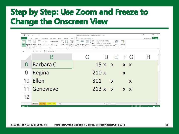
Step by Step: Use Zoom and Freeze to Change the Onscreen View • USE the workbook from the previous exercise. 1. Maximize the window containing the Monday worksheet. 2. SAVE the workbook in the Excel Lesson 8 folder as 08 Spa Services Week of 2 -20 Solution 3. 3. Select cell B 8. 4. To increase magnification, click and hold the zoom control in the lower-right corner and slide the pointer to the right (see the figure on the next slide). The maximum zoom is 400%. Notice the window zooms in on the selected cell. © 2016, John Wiley & Sons, Inc. Microsoft Official Academic Course, Microsoft Excel Core 2016 35

Step by Step: Use Zoom and Freeze to Change the Onscreen View © 2016, John Wiley & Sons, Inc. Microsoft Official Academic Course, Microsoft Excel Core 2016 36

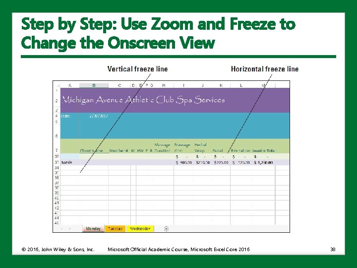
Step by Step: Use Zoom and Freeze to Change the Onscreen View 5. Click the View tab, and in the Zoom group, click 100%. The worksheet returns to standard magnification. Scroll to the top of the worksheet so that row 1 is visible again. If you need to, scroll left so you can also see column A again. 6. Select cell B 8 again, if necessary. On the View tab, in the Window group, click Freeze Panes and then click Freeze Panes in the menu that appears. Cells above and to the left of the selected cell (B 8) are now frozen in place for scrolling. 7. Scroll down so that row 33 comes close to the labels in row 7. Notice that rows 1 through 7 remain in place (see the figure on the next slide). © 2016, John Wiley & Sons, Inc. Microsoft Official Academic Course, Microsoft Excel Core 2016 37

Step by Step: Use Zoom and Freeze to Change the Onscreen View © 2016, John Wiley & Sons, Inc. Microsoft Official Academic Course, Microsoft Excel Core 2016 38

Step by Step: Use Zoom and Freeze to Change the Onscreen View 8. Press Ctrl+Home to scroll the worksheet to the top. On the View tab, in the Window group, click Freeze Panes and then click Unfreeze Panes. The thin lines denoting the frozen borders of the worksheet disappear. • LEAVE the workbook open to use in the next exercise. • You can use hold down the Ctrl key and use the wheel of your mouse to zoom in (up) and out (down) of a worksheet. © 2016, John Wiley & Sons, Inc. Microsoft Official Academic Course, Microsoft Excel Core 2016 39

Finding and Replacing Data • Excel has a Find command a Replace command that work similarly to Microsoft Word, only they navigate through cells instead of paragraphs. • You can use the Find command to search for text you’ve entered as data, such as a person’s name, as well as values that happen to be the results of formulas. © 2016, John Wiley & Sons, Inc. Microsoft Official Academic Course, Microsoft Excel Core 2016 40

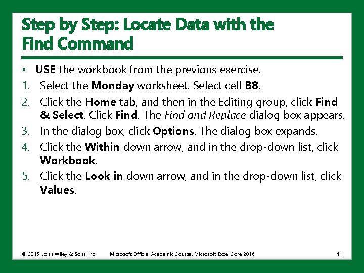
Step by Step: Locate Data with the Find Command • USE the workbook from the previous exercise. 1. Select the Monday worksheet. Select cell B 8. 2. Click the Home tab, and then in the Editing group, click Find & Select. Click Find. The Find and Replace dialog box appears. 3. In the dialog box, click Options. The dialog box expands. 4. Click the Within down arrow, and in the drop-down list, click Workbook. 5. Click the Look in down arrow, and in the drop-down list, click Values. © 2016, John Wiley & Sons, Inc. Microsoft Official Academic Course, Microsoft Excel Core 2016 41

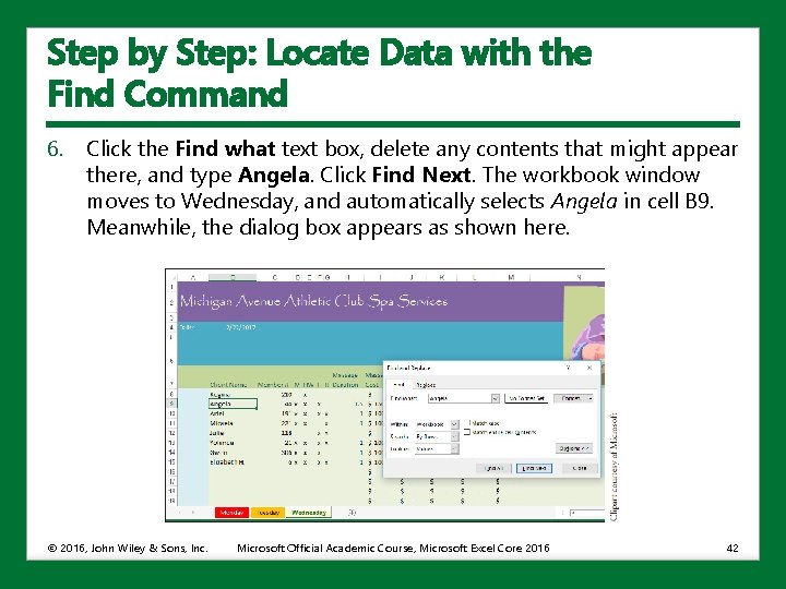
Step by Step: Locate Data with the Find Command 6. Click the Find what text box, delete any contents that might appear there, and type Angela. Click Find Next. The workbook window moves to Wednesday, and automatically selects Angela in cell B 9. Meanwhile, the dialog box appears as shown here. © 2016, John Wiley & Sons, Inc. Microsoft Official Academic Course, Microsoft Excel Core 2016 42

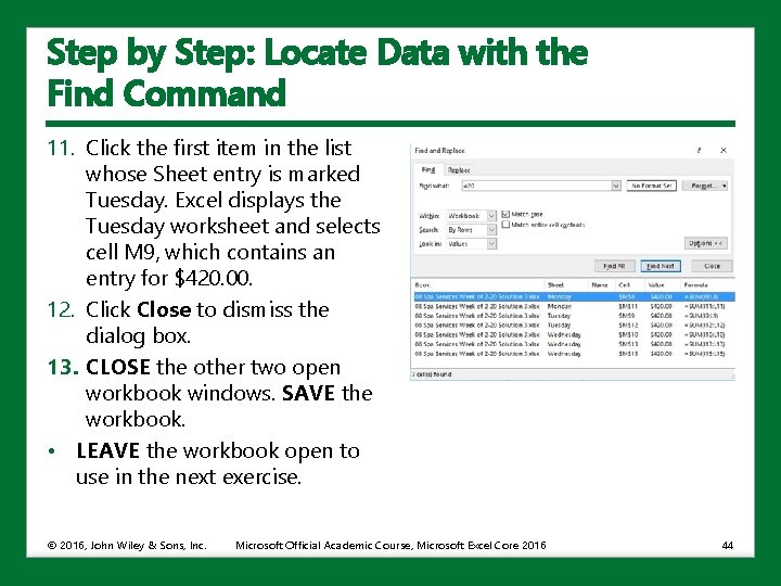
Step by Step: Locate Data with the Find Command 7. Double-click the Find what text box, press Delete, and then type Beth. Click Find Next. Excel highlights cell B 15, whose contents include “beth” in the middle of the cell and in a non-matching case. 8. Select cell B 9. 9. In the dialog box, click Match case and then click Find Next. This time, Excel reports the text can’t be found, because it’s looking for a name that begins with a capital “B. ” Click OK to dismiss the message. 10. Double-click the Find what text box, press Delete, and then type 420. Click Find All. The dialog box shows a detailed report listing all the cells in the workbook that contain the value 420. In this case, it points to all the locations where customers paid “the works” for all the services together. You can use the scroll bars or drag the lower-right corner of the dialog box to see all the data, see the figure on the next slide. © 2016, John Wiley & Sons, Inc. Microsoft Official Academic Course, Microsoft Excel Core 2016 43

Step by Step: Locate Data with the Find Command 11. Click the first item in the list whose Sheet entry is marked Tuesday. Excel displays the Tuesday worksheet and selects cell M 9, which contains an entry for $420. 00. 12. Click Close to dismiss the dialog box. 13. CLOSE the other two open workbook windows. SAVE the workbook. • LEAVE the workbook open to use in the next exercise. © 2016, John Wiley & Sons, Inc. Microsoft Official Academic Course, Microsoft Excel Core 2016 44

Replacing Data with the Replace Command • The functions for finding and for replacing text are located in the same dialog box. • Excel gives you two ways to bring this dialog box up. • You might have already noticed the Find tab at the top of the Find and Replace dialog box. The Replace tab is next to it. • The Replace command adds a text box for the contents you intend to insert in place of any matches Excel finds. © 2016, John Wiley & Sons, Inc. Microsoft Official Academic Course, Microsoft Excel Core 2016 45

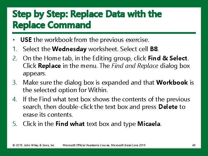
Step by Step: Replace Data with the Replace Command • USE the workbook from the previous exercise. 1. Select the Wednesday worksheet. Select cell B 8. 2. On the Home tab, in the Editing group, click Find & Select. Click Replace in the menu. The Find and Replace dialog box appears. 3. Make sure the dialog box is expanded and that Workbook is the selected option for Within. 4. If the Find what text box shows the contents of the previous search, then double-click the text box and press Delete to erase its contents. 5. Click in the Find what text box and type Micaela. © 2016, John Wiley & Sons, Inc. Microsoft Official Academic Course, Microsoft Excel Core 2016 46

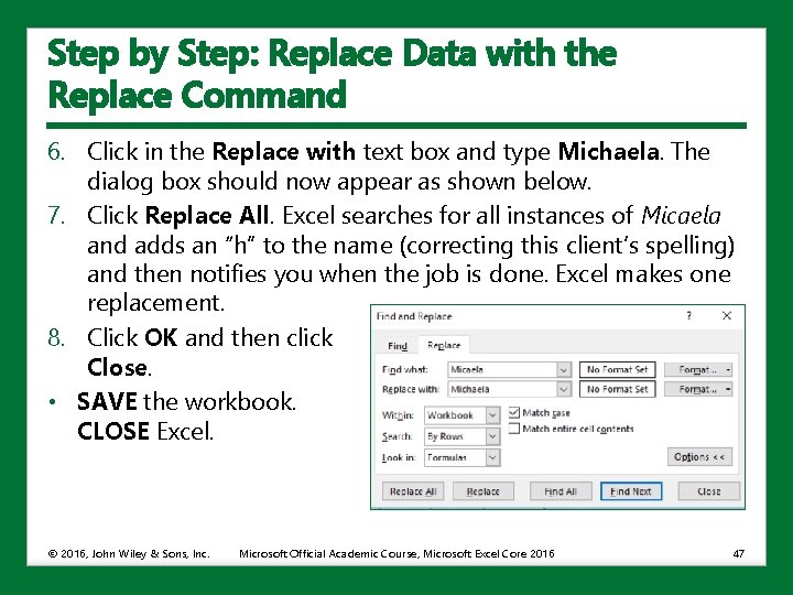
Step by Step: Replace Data with the Replace Command 6. Click in the Replace with text box and type Michaela. The dialog box should now appear as shown below. 7. Click Replace All. Excel searches for all instances of Micaela and adds an “h” to the name (correcting this client’s spelling) and then notifies you when the job is done. Excel makes one replacement. 8. Click OK and then click Close. • SAVE the workbook. CLOSE Excel. © 2016, John Wiley & Sons, Inc. Microsoft Official Academic Course, Microsoft Excel Core 2016 47

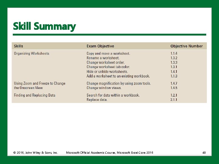
Skill Summary © 2016, John Wiley & Sons, Inc. Microsoft Official Academic Course, Microsoft Excel Core 2016 48