Excel 2010 Training Microsoft Excel is a popular

Excel 2010 Training Microsoft Excel is a popular spreadsheet program that is part of the Microsoft Office suite of products. This Training document deals with Excel 2010, the latest version of Excel.

Goals • Upon completion of this 1 -on-1 training, you will be able to: • Create a Workbook • Make Basic Formatting Changes • Save and Print a Workbook • Save a Workbook For Use With Previous Versions of Excel • Customize the Ribbon

Enhancements in Excel 2010 • • • File Menu Returns: The Windows button of Office 2007 has been replaced with an updated File menu, which, when clicked, takes you to the new Backstage View. See URL for details. Updated Ribbon: It is now possible to customize the Ribbon to suit your personal needs and preferences. Sparklines: Sparklines are essentially miniature graphs that fit inside a single cell of a table. They can provide concise visual summaries of data such as investment performance. Slicers: Slicers are a new easy way to filter your data interactively. They can be hooked up to Pivot. Tables or Pivot. Charts as intuitive interfaces for reports. Power. Pivot for Excel: Power. Pivot is a data analysis tool that runs within Excel 2010. This lets you use Excel features, such as Pivot. Tables and slicers, to analyze large quantities of data almost instantly. Screenshot Tool: Excel now has a built-in screen capture utility, so you don’t have to open up Snip to take screenshots. You can use this utility to capture images of any window you have open, not just Excel. Photo Editing: Excel’s built-in photo editing capabilities are more powerful in Excel 2010. For example, you can change the color saturation or invert the picture, and you can see thumbnail previews of photo edits before you make them. Paste Preview: You can use Paste Preview to see how the different types of pasting will affect the look of the document before actually pasting material in. Web Apps: Microsoft Office now has online functionality similar to that of Norse Docs. You can access documents from any computer connected to the Internet, share them with others, and even open them on a mobile phone.

Create a Workbook A file that you create with Excel is called a “workbook”. A workbook is a set of spreadsheets called “worksheets”. First, open Microsoft Excel by clicking Start > All Programs > Applications > Microsoft Office Excel 2010. — Note: Excel may be located in a different place in your Start menu.

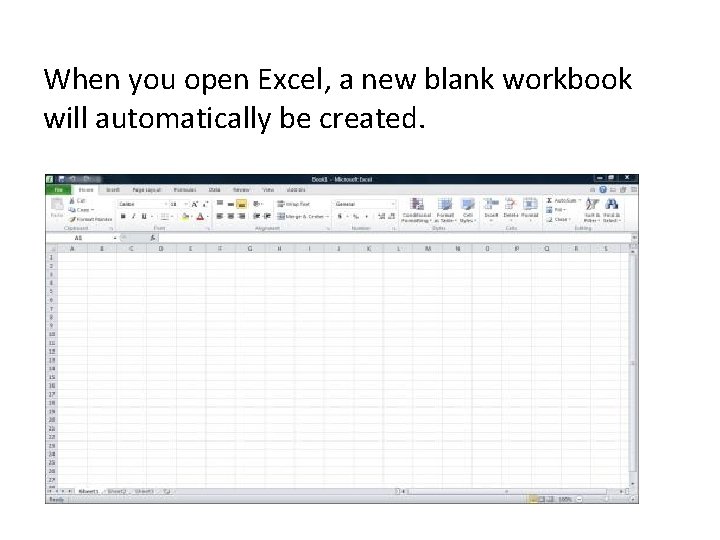
When you open Excel, a new blank workbook will automatically be created.

Enter Data into a Worksheet A worksheet is a grid array of cells, into which you can enter data. The columns are lettered, and the rows are numbered. A cell can be referred to by its “reference”, which is its column letter followed by its row number. For example, A 1 is the top left cell. The basic process for entering data into a cell is to select a cell, and start typing data into it. A selected cell has a black rectangle around it. Let’s enter some simple data into our spreadsheet.

1. Click on cell B 1 to select it. Type “Price, ” and hit the Tab button. — Note: when you hit the Tab button after entering data, you move one cell to the right. 2. Type “Qty” in cell C 1, hit Tab, and type “Ext Price” in cell D 1. 3. Select cell A 2, type “Whizbang, ” and hit Enter. — Note: when you hit Enter, you move one cell down. 4. In cell A 3, type “Gadget. ” In cell A 4, type “Gizmo. ” In cell A 5, type “Red Stapler. ”

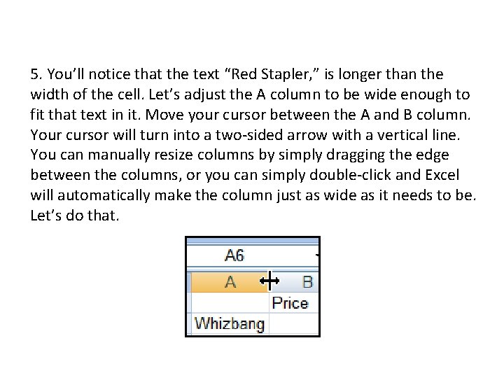
5. You’ll notice that the text “Red Stapler, ” is longer than the width of the cell. Let’s adjust the A column to be wide enough to fit that text in it. Move your cursor between the A and B column. Your cursor will turn into a two-sided arrow with a vertical line. You can manually resize columns by simply dragging the edge between the columns, or you can simply double-click and Excel will automatically make the column just as wide as it needs to be. Let’s do that.

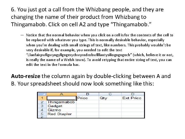
6. You just got a call from the Whizbang people, and they are changing the name of their product from Whizbang to Thingamabob. Click on cell A 2 and type “Thingamabob. ” — Notice that the normal behavior when you click on a cell is for the contents of the cell to be replaced with whatever you type. This is normally desirable behavior, especially when you’re dealing with small strings of text, like numbers. This probably wouldn’t be very desirable if, for example, you needed to edit the text “Llanfairpwllgwyngyllgogerychwyrndrobwllllantysiliogogogoch” (which, believe it or not, is really the name of a Welsh town). To avoid retyping that entire string of text, you can edit the text in the Formula bar. Auto-resize the column again by double-clicking between A and B. Your spreadsheet should now look something like this:

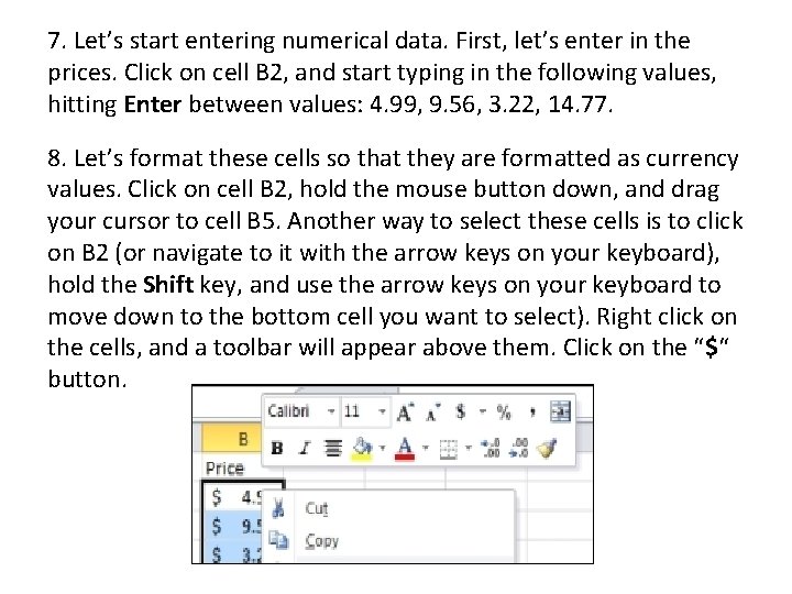
7. Let’s start entering numerical data. First, let’s enter in the prices. Click on cell B 2, and start typing in the following values, hitting Enter between values: 4. 99, 9. 56, 3. 22, 14. 77. 8. Let’s format these cells so that they are formatted as currency values. Click on cell B 2, hold the mouse button down, and drag your cursor to cell B 5. Another way to select these cells is to click on B 2 (or navigate to it with the arrow keys on your keyboard), hold the Shift key, and use the arrow keys on your keyboard to move down to the bottom cell you want to select). Right click on the cells, and a toolbar will appear above them. Click on the “$“ button.

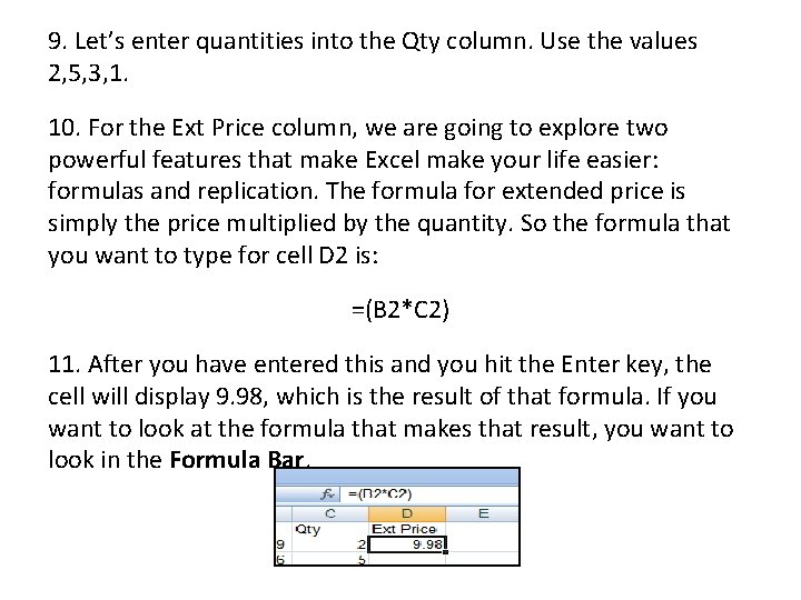
9. Let’s enter quantities into the Qty column. Use the values 2, 5, 3, 1. 10. For the Ext Price column, we are going to explore two powerful features that make Excel make your life easier: formulas and replication. The formula for extended price is simply the price multiplied by the quantity. So the formula that you want to type for cell D 2 is: =(B 2*C 2) 11. After you have entered this and you hit the Enter key, the cell will display 9. 98, which is the result of that formula. If you want to look at the formula that makes that result, you want to look in the Formula Bar.

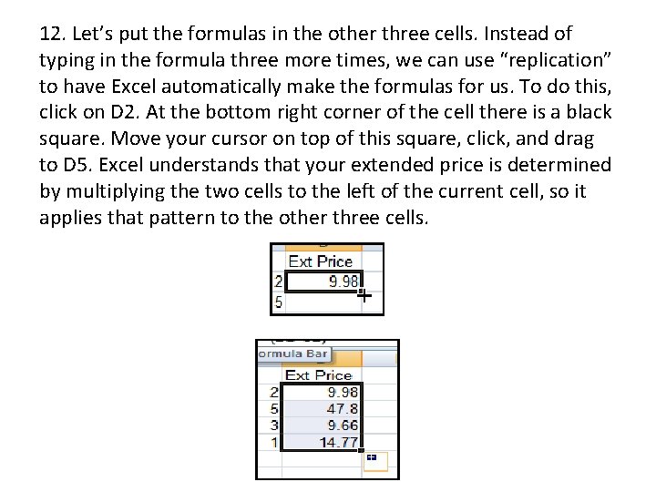
12. Let’s put the formulas in the other three cells. Instead of typing in the formula three more times, we can use “replication” to have Excel automatically make the formulas for us. To do this, click on D 2. At the bottom right corner of the cell there is a black square. Move your cursor on top of this square, click, and drag to D 5. Excel understands that your extended price is determined by multiplying the two cells to the left of the current cell, so it applies that pattern to the other three cells.

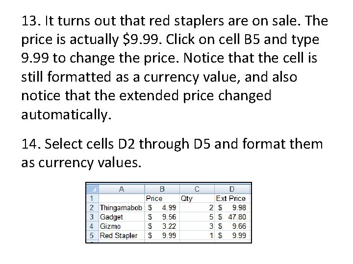
13. It turns out that red staplers are on sale. The price is actually $9. 99. Click on cell B 5 and type 9. 99 to change the price. Notice that the cell is still formatted as a currency value, and also notice that the extended price changed automatically. 14. Select cells D 2 through D 5 and format them as currency values.

Format Cells as Table One of Excel 2010’s new features is the ability to quickly format a series of cells as a table. With a couple of clicks, you can take some boring looking data and make it semi-exciting. We are going to do this to the data we entered earlier.

1. Select cells A 1 through D 5 by clicking on A 1, holding the Shift key, and clicking on D 5. — Note: you can also select a range of cells by holding the Shift key and using arrows on your keyboard. 2. Click the Format as Table button in the Ribbon, and choose that nice medium green colored table. A dialog box will pop up, asking you where your data is. Click OK. 3. In the Ribbon, you’ll notice that Table Tools have appeared, because you’re working on a table. Put a check mark on the Total Row option. 4. To give a little bit of distinction to the products in our invoice, let’s also place a check mark on First Column. This makes the product names bold.

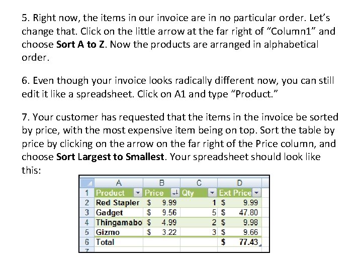
5. Right now, the items in our invoice are in no particular order. Let’s change that. Click on the little arrow at the far right of “Column 1” and choose Sort A to Z. Now the products are arranged in alphabetical order. 6. Even though your invoice looks radically different now, you can still edit it like a spreadsheet. Click on A 1 and type “Product. ” 7. Your customer has requested that the items in the invoice be sorted by price, with the most expensive item being on top. Sort the table by price by clicking on the arrow on the far right of the Price column, and choose Sort Largest to Smallest. Your spreadsheet should look like this:

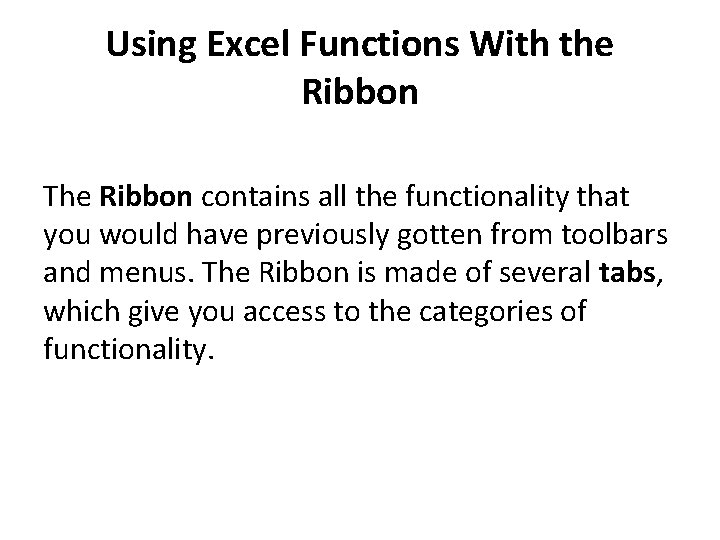
Using Excel Functions With the Ribbon The Ribbon contains all the functionality that you would have previously gotten from toolbars and menus. The Ribbon is made of several tabs, which give you access to the categories of functionality.

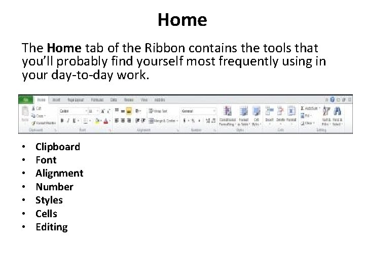
Home The Home tab of the Ribbon contains the tools that you’ll probably find yourself most frequently using in your day-to-day work. • • Clipboard Font Alignment Number Styles Cells Editing

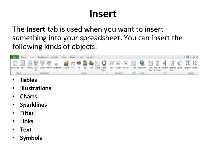
Insert The Insert tab is used when you want to insert something into your spreadsheet. You can insert the following kinds of objects: • • Tables Illustrations Charts Sparklines Filter Links Text Symbols

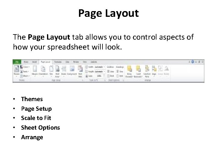
Page Layout The Page Layout tab allows you to control aspects of how your spreadsheet will look. • • • Themes Page Setup Scale to Fit Sheet Options Arrange

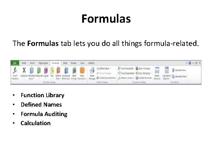
Formulas The Formulas tab lets you do all things formula-related. • • Function Library Defined Names Formula Auditing Calculation

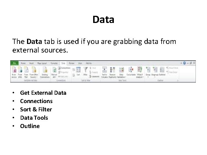
Data The Data tab is used if you are grabbing data from external sources. • • • Get External Data Connections Sort & Filter Data Tools Outline

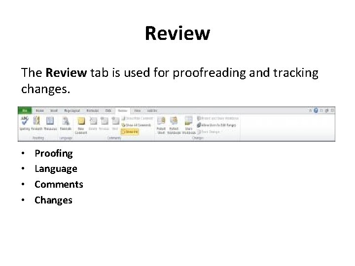
Review The Review tab is used for proofreading and tracking changes. • • Proofing Language Comments Changes

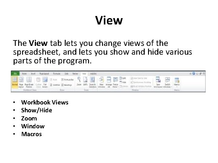
View The View tab lets you change views of the spreadsheet, and lets you show and hide various parts of the program. • • • Workbook Views Show/Hide Zoom Window Macros

Save Workbook In Excel 2010 (and other Office programs), the Office Button has been replaced with the File tab. This tab gives you access to things that you used to find in the Office Button, or the file menu in earlier versions, like opening, saving and printing, and it also gives you access to Excel options. The file tab also shows a backstage view of a document. The Backstage view is where you manage your documents and related data about them To save, click the File tab, and click Save. You can also use the Ctrl+S keyboard shortcut.

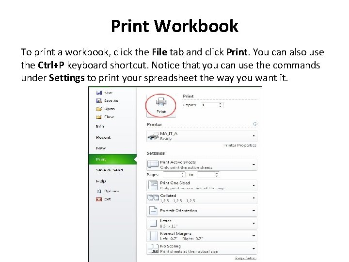
Print Workbook To print a workbook, click the File tab and click Print. You can also use the Ctrl+P keyboard shortcut. Notice that you can use the commands under Settings to print your spreadsheet the way you want it.

Save a Workbook for Use With Previous Versions of Excel 97, Excel 2000, Excel XP, and Excel 2003 all saved files in the same file format. Office 2010 continues to use the office 2007 file format based on XML. This file format makes for smaller files that are more human-readable, and are less likely to become corrupted. However, previous version of Office cannot open files in the new format without an add-on. If you need to share files with somebody who doesn’t have Office 2010 and doesn’t have the needed add-on, you may save your document in the older format. However, if you use any Excel 2010 -specific features in this document, they’ll be lost in translation. — The add-on from Microsoft is available here.

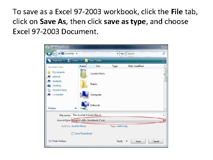
To save as a Excel 97 -2003 workbook, click the File tab, click on Save As, then click save as type, and choose Excel 97 -2003 Document.

Customize the Ribbon Excel and other 2010 Office programs give you the option to customize the Ribbon in order to have quick access to commands you use most often, such as save, or cut. Now let’s say you want to have the Quick print command right under your eyes for easy access. To do this: 1. Click on the File tab, then click Options, and select Customize Ribbon. 2. In the box on the right labeled Customize the Ribbon assure Main Tabs is selected. 3. The box below will now read Main Tabs. Select Home, then click on New Group at the bottom of the page. 4. The title New Group (Custom) immediately pops under the tab Home. You can click on Rename and call it whatever you want.

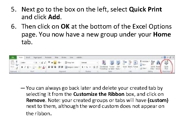
5. Next go to the box on the left, select Quick Print and click Add. 6. Then click on OK at the bottom of the Excel Options page. You now have a new group under your Home tab. — You can always go back later and delete your created tab by selecting it from the Customize the Ribbon box, and click on Remove. Note: your created groups or tabs will have (custom) next to them, although the word custom does not appear on the ribbon.

Additional Resources Review the Help within Excel 2010 has a built-in help system. Hit the F 1 key, or click the question mark on the upper right part of the window to access it. – You can select a topic by clicking on the text, such as Getting Started with Excel 2010. – You can also type a word or phrase into the box at the top of the window, click the Search button, and then select the topic of interest.

Additional Resources Cont Review the Technology Help Desk web site and Project Page for additional • www. baruch. cuny. edu/bctc BCTC Help Desk • Call 646 -312 -1010 • Email helpdesk@baruch. cuny. edu • Visit the BCTC Help Desk on the 6 th Floor of the Library Building