Managerial Economics Lecture Eleven Alternative theories of finance

Managerial Economics Lecture Eleven: Alternative theories of finance

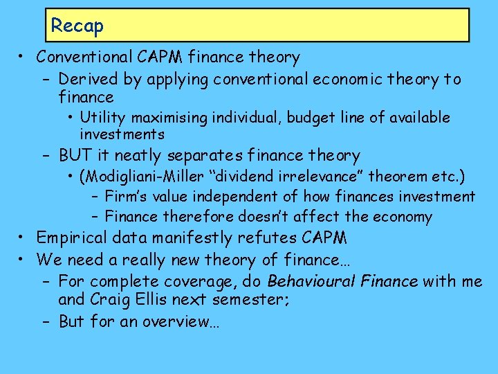
Recap • Conventional CAPM finance theory – Derived by applying conventional economic theory to finance • Utility maximising individual, budget line of available investments – BUT it neatly separates finance theory • (Modigliani-Miller “dividend irrelevance” theorem etc. ) – Firm’s value independent of how finances investment – Finance therefore doesn’t affect the economy • Empirical data manifestly refutes CAPM • We need a really new theory of finance… – For complete coverage, do Behavioural Finance with me and Craig Ellis next semester; – But for an overview…

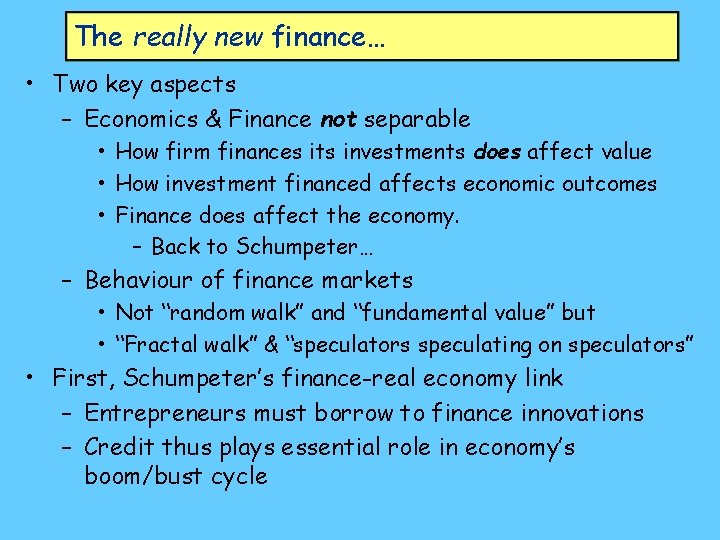
The really new finance… • Two key aspects – Economics & Finance not separable • How firm finances its investments does affect value • How investment financed affects economic outcomes • Finance does affect the economy. – Back to Schumpeter… – Behaviour of finance markets • Not “random walk” and “fundamental value” but • “Fractal walk” & “speculators speculating on speculators” • First, Schumpeter’s finance-real economy link – Entrepreneurs must borrow to finance innovations – Credit thus plays essential role in economy’s boom/bust cycle

Schumpeter’s model: money has real effects • In Schumpeter’s model, entrepreneurs start new firms – No retained earnings, capital, workers • “…the carrying out of new combinations takes place through the withdrawal of services of labor and land from their previous employments… • this again leads us to … the heresy that money, and … other means of payment, perform an essential function, – hence that processes in terms of means of payment are not merely reflexes of processes in terms of goods. • In every possible strain, with rare unanimity, even with impatience and moral and intellectual indignation, a very long line of theorists have assured us of the opposite. ” (Schumpeter p. 95)

Schumpeter’s model: money has real effects • Conventional interpretation of money emphasises – Money simply a “veil over barter” – Money plays no essential role • Double all prices & incomes, no-one better or worse off • Schumpeter accepts above as true for existing products, production techniques, etc. , in general equilibrium • But new products, new methods, disturb “the circular flow”. Money plays essential role in this disequilibrium phenomenon – Affects the price level and output – Doubling all prices & incomes would make some better off, some worse • Those with debts would be better off – Including entrepreneurs…

Schumpeter’s model: money has real effects • Conventional theory suffers from “barter illusion” – Existing producers using existing production methods exchanging existing products • “Walras’ Law” applies • Major role of finance is initiating new products / production methods etc. ; • For these equilibrium-disturbing events, classic “money a veil over barter” concept cannot apply. – “From this it follows, therefore, that in real life total credit must be greater than it could be if there were only fully covered credit. The credit structure projects not only beyond the existing gold basis, but also beyond the existing commodity basis. ” (101) • “Walras’ Law” therefore false for growing economy…

Schumpeter’s model: credit has real effects • “[T]he entrepreneur needs credit … • [T]his purchasing power does not flow towards him automatically, as to the producer in the circular flow, by the sale of what he produced in preceding periods. • If he does not happen to possess it … he must borrow it… He can only become an entrepreneur by previously becoming a debtor… • his becoming a debtor arises from the necessity of the case and is not something abnormal, an accidental event to be explained by particular circumstances. What he first wants is credit. Before he requires any goods whatever, he requires purchasing power. He is the typical debtor in capitalist society. ” (102)

Schumpeter’s model: credit has real effects • In normal productive cycle, income from production finances purchases; credit can be used, but not essential – “[T]he decisive point is that we can, without overlooking anything essential, represent the process within the circular flow as if production were currently financed by receipts. ” (104) • Effectively, Say’s Law applies: “supply creates its own demand” • Aggregate demand equals aggregate supply (with maybe some sectors above, some sectors below) – But credit-financed entrepreneurs very different • Expenditure (demand) not financed by current receipts (supply) but by credit • Aggregate Demand exceeds Aggregate Supply

Schumpeter’s model: credit has real effects • Credit finance for entrepreneurs thus endogenous: not “deposits create loans” but “loans create deposits”: – “[I]n so far as credit cannot be given out of the results of past enterprise … it can only consist of credit means of payment created ad hoc, which can be backed neither by money in the strict sense nor by products already in existence. . . – It provides us with the connection between lending and credit means of payment, and leads us to what I regard as the nature of the credit phenomenon. ” (106)

Schumpeter’s model: credit has real effects • “[G]iving credit involves creating purchasing power, and newly created purchasing power is of use only in giving credit to the entrepreneur, … credit is essentially the creation of purchasing power for the purpose of transferring it to the entrepreneur, but not simply the transfer of existing purchasing power. • The creation of purchasing power characterises, in principle, the method by which development is carried out in a system with private property and division of labor. • By credit, entrepreneurs are given access to the social stream of goods before they have acquired the normal claim to it. ” (106 -107) • Credit irrelevant to equilibrium economics, but essential to disequilibrium process of economic development:

Schumpeter’s model: credit has real effects • “… credit is not essential in the normal circular flow, because … it can be assumed there that all purchases of production goods by producers are cash transactions or that in general whoever is a buyer previously sold goods of the same money value…” • However “it is certain that there is such a gap to bridge in the carrying out of new combinations. To bridge it is the function of the lender, and he fulfils it by placing purchasing power created ad hoc at the disposal of the entrepreneur. • Then those who supply production goods need not "wait" and yet the entrepreneur need advance them neither goods nor existing money. Thus the gap is closed which would otherwise make development extraordinarily difficult, if not impossible in an exchange economy where private property prevails. ” (107) • So process of innovation & change breaches Say’s Law: in growing, changing economy – Demand exceeds receipts from current sales – Difference financed by credit (debt) to entrepreneurs

Schumpeter’s model: credit has real effects • Say’s Law & Walras’ Law apply in circular flow, but not entrepreneurial credit-financed activity: – “In the circular flow, from which we always start, the same products are produced every year in the same way. For every supply there waits somewhere in the economic system a corresponding demand, for every demand the corresponding supply. All goods are dealt in at determined prices with only insignificant oscillations, so that every unit of money may be considered as going the same way in every period. A given quantity of purchasing power is available at any moment to purchase the existing quantity of original productive services, in order then to pass into the hands of their owners and then again to be spent on consumption goods. ” (108)

Aside: “Marx with different adjectives” • Schumpeter’s thinking here very similar to Marx – Marx argued there were two “Circuits of Capital” • Commodity—Money—Commodity – Equivalent to Schumpeter’s “circular flow” – Essentially Say’s Law applies • Sellers only sell in order to buy • Money—Commodity—Money – Equivalent to Schumpeter’s entrepreneurial function • Schumpeter’s – Say’s Law doesn’t apply: “The capitalist throws less value in the form of money into the circulation than point: • Capitalist “throws he draws out of it. . . Since he functions. . . as an in” borrowed money industrial capitalist, his supply of commodity-value is always greater than his demand for it. If his supply • Succeeds if can and demand in this respect covered each other it repay debt and would mean that his capital had not produced any pocket some of the surplus-value. . . His aim is not to equalize his supply gap and demand, but to make the inequality between them. . . as great as possible. ” (Marx 1885: 120 -121)

Schumpeter’s model: credit has real effects • “If now credit means of payment … are created and placed at the entrepreneur's disposal, then … his purchasing power [takes] its place beside the total previously existing. • Obviously this does not increase the quantity of productive services existing in the economic system. Yet "new demand" becomes possible in a very obvious sense. • It causes a rise in the prices of productive services. From this ensues the "withdrawal of goods" from their previous use…” (108) – Aggregate Demand exceeds Aggregate Supply; Say’s Law violated in move from stationary state • Sum of excess demands negative (not zero as in Walras’ Law) – Credit-financed demand a source of price inflation…

Schumpeter’s model: credit has real effects • “Just as when additional gas streams into a vessel the share of the space occupied by each molecule of the previously existing gas is diminished by compression, so the inflow of new purchasing power into the economic system will compress the old purchasing power. • When the price changes which thus become necessary are completed, any given commodities exchange for the new units of purchasing power on the same terms as for the old, only the units of purchasing power now existing are all smaller than those existing before and their distribution among individuals has been shifted. ” (109) • This inflation – Isn’t necessarily a bad thing – Can be reversed by dynamics of economic development

Schumpeter’s model: credit has real effects • “credit inflation. . is distinguished from … inflation for consumptive purposes by a very essential element… • The entrepreneur must not only legally repay money to his banker, but he must also economically repay commodities to the reservoir of goods … • after a period at the end of which his products are on the market and his productive goods used up - he has, if everything has gone according to expectations, enriched the social stream with goods whose total price is greater than the credit received and than the total price of the goods directly and indirectly used up by him. • Hence the equivalence between the money and commodity streams is more than restored, the credit inflation more than eliminated, the effect upon prices more than compensated for. ” (110)

Schumpeter’s model: credit has real effects • “Furthermore, the entrepreneur can now repay his debt (amount credited plus interest) at his bank, and normally still retain a credit balance (= entrepreneurial profit) that is withdrawn from the purchasing-power fund of the circular flow. ” (111) • So dynamic view of economy – Overturns “money doesn’t have real effects” bias of neoclassicals/monetarists – Breaches “supply creates its own demand” Say’s Law view of self-equilibrating economy – Breaches Walras’ Law “if n-1 markets in equilibrium, nth also in equilibrium” general equilibrium analysis – Links finance and economics: without finance there would not be economic growth, but – Finance can affect economic growth negatively as well as positively (if entrepreneurial expectations fail)…

The really new finance… • Dynamic vision of economics overturns equilibrium truths • Ditto realistic view of finance markets: not equilibrium but disequilibrium dynamics… • Three highly unrealistic assumptions essential to CAPM: – Investors agree on values of all shares – Perceptions of values are correct – All investors have limitless access to risk free finance • Outcome: shares follow “random walk” • Really new finance rejects all these assumptions: – Investors disagree on values of shares – Future uncertain & perceptions of future wrong – Differing access to finance • Outcome: shares follow “fractal walk”

The really new finance… • Several as yet not integrated aspects – Behavioural Finance • Investors don’t make “rational utility maximising” decisions when confronted with risky financial choices – Inefficient Finance • Finance markets themselves not efficient – “Minority Game” • Financial Markets as game in which you win by being in the minority – Fractal Finance • Statistical properties of markets “fractal” and “power law”, not random – Last (empirical) aspect first…

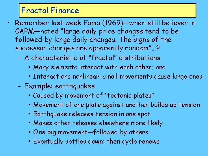
Fractal Finance • Remember last week Fama (1969)—when still believer in CAPM—noted “large daily price changes tend to be followed by large daily changes. The signs of the successor changes are apparently random”…? – A characteristic of “fractal” distributions • Many elements interact with each other; and • Interactions nonlinear: small movements cause large ones – Example: earthquakes • • • Caused by movement of “tectonic plates” Movement of one plate against another builds up tension Earthquake releases tension in one spot Makes other releases elsewhere more likely One big movement—followed by others Eventually settles down; then cycle renews

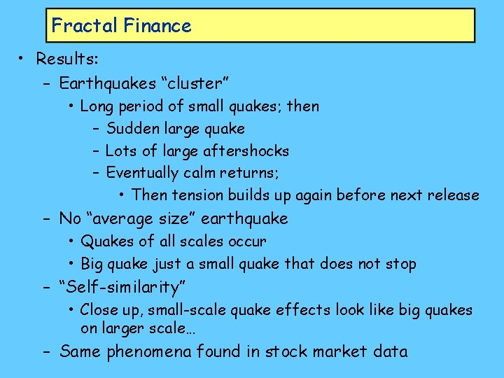
Fractal Finance • Results: – Earthquakes “cluster” • Long period of small quakes; then – Sudden large quake – Lots of large aftershocks – Eventually calm returns; • Then tension builds up again before next release – No “average size” earthquake • Quakes of all scales occur • Big quake just a small quake that does not stop – “Self-similarity” • Close up, small-scale quake effects look like big quakes on larger scale… – Same phenomena found in stock market data

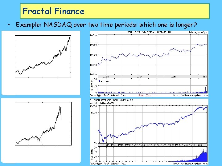
Fractal Finance • Volatility clustering – Periods of high volatility not randomly distributed but clustered together • No “average” size daily/weekly/yearly movement – Averages & standard deviations can be calculated • But data does not fit means, deviations etc. – Highly skewed – Many more large events than predicted • Self-similarity – Intra-day pattern in a day looks like – Daily pattern in a month – Monthly pattern in a decade…

Fractal Finance • Example: NASDAQ over two time periods: which one is longer?

Fractal Finance • What’s the point? – Randomly generated pattern would have decreasing volatility as time scale increased: • Variance of random distribution scales to square root of time scale • Variance of actual financial time series scales linearly with time • No “average” scale of movement at any time scale: – Random distribution: huge movements can be ruled out – Actual financial time series: huge movements can and do occur: • 10% fall of DJIA on “Black Friday” in 1929 • 25% fall of ASX on “Black Tuesday” in 1987 • 14% fall of NASDAQ in April 2000…

Fractal Finance • “If we take a graph of the S&P 500 index …, and place it above a graph of an uncorrelated biased random walk with the same overall bias, at first glance they seem almost identical. • When we look closer, however, we notice the graph of the S&P 500 has occasional large fluctuations (e. g. the huge drop that took place on Black Monday in October, 1987 (when most world markets lost 20 -30% of their value over a period of 1 -2 days). • We do not see this kind of large fluctuation in the biased random walk graph because the probability of taking a very large number of random steps in the same direction (which would be necessary for a large fluctuation) is exponentially small. ” (Stanley, Physica A 2000: 9)

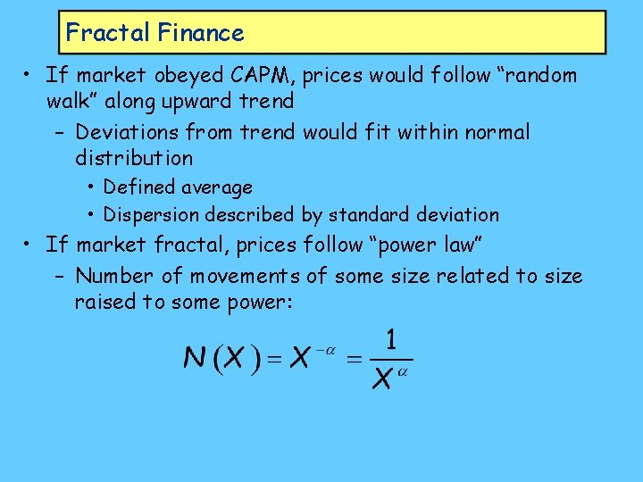
Fractal Finance • If market obeyed CAPM, prices would follow “random walk” along upward trend – Deviations from trend would fit within normal distribution • Defined average • Dispersion described by standard deviation • If market fractal, prices follow “power law” – Number of movements of some size related to size raised to some power:

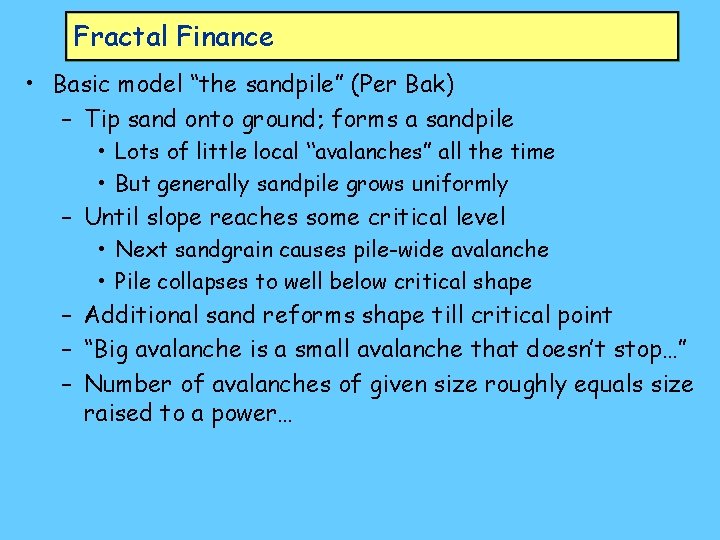
Fractal Finance • Basic model “the sandpile” (Per Bak) – Tip sand onto ground; forms a sandpile • Lots of little local “avalanches” all the time • But generally sandpile grows uniformly – Until slope reaches some critical level • Next sandgrain causes pile-wide avalanche • Pile collapses to well below critical shape – Additional sand reforms shape till critical point – “Big avalanche is a small avalanche that doesn’t stop…” – Number of avalanches of given size roughly equals size raised to a power…

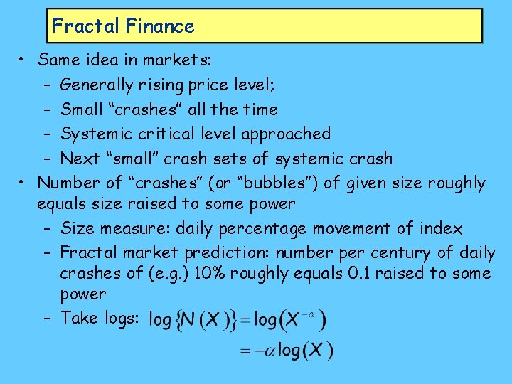
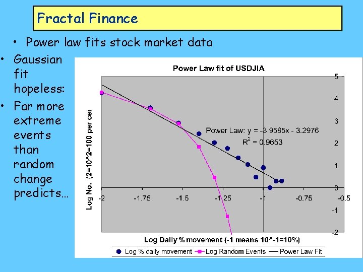
Fractal Finance • Same idea in markets: – Generally rising price level; – Small “crashes” all the time – Systemic critical level approached – Next “small” crash sets of systemic crash • Number of “crashes” (or “bubbles”) of given size roughly equals size raised to some power – Size measure: daily percentage movement of index – Fractal market prediction: number per century of daily crashes of (e. g. ) 10% roughly equals 0. 1 raised to some power – Take logs:

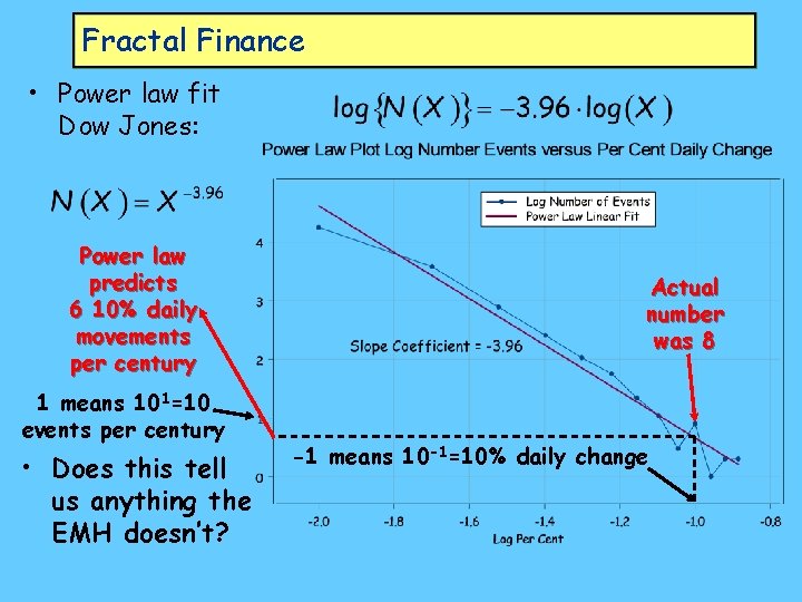
Fractal Finance • Power law fit Dow Jones: Power law predicts 6 10% daily movements per century 1 means 101=10 events per century • Does this tell us anything the EMH doesn’t? Actual number was 8 -1 means 10 -1=10% daily change

Fractal Finance • Power law fits stock market data • Gaussian fit hopeless: • Far more extreme events than random change predicts…

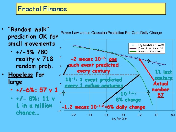
Fractal Finance • “Random walk” prediction OK for small movements • +/-3% 780 -2 means 10 -2: one reality v 718 such event predicted random prob. every century • Hopeless for -6: 1 event predicted 10 large every 1 million centuries • +/-6%: 57 v 1 10 -1. 1: • +/- 8%: 11 v 8% change 1 in a million -1. 2 means 10 -1. 2=6% daily change chance… 11 last century Actual number 57

Fractal Finance • Other statistical properties found: – “Tsallis’s q” – Sornette’s “Log-periodic” crashes… • Most research done by physicists (“econophysicists”) • Characterise how the market behaves – Large movements – Clearly interactions between agents • Like interactions between grains of sand in sandpile—one grain pushes several others that push others… chain reaction to avalanche • Doesn’t explain why market behaves this way • Over to “behavioural finance”…

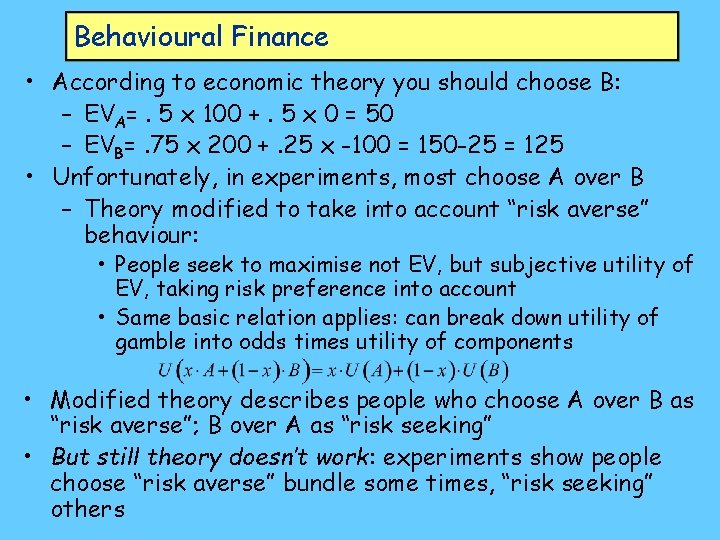
Behavioural Finance • CAPM based on “rational utility maximising behaviour” • Expected utility hypothesis: – Given two risky outcomes, agent chooses one that maximises expected value: • Problem 1: You have to choose between two alternatives: – A: 50% chance of $100 and 50% chance of nothing – B: 75% chance of $200 and 25% chance of -$100 • Which would you choose? . . . • Write your choice down: – A or B?

Behavioural Finance • According to economic theory you should choose B: – EVA=. 5 x 100 +. 5 x 0 = 50 – EVB=. 75 x 200 +. 25 x -100 = 150 -25 = 125 • Unfortunately, in experiments, most choose A over B – Theory modified to take into account “risk averse” behaviour: • People seek to maximise not EV, but subjective utility of EV, taking risk preference into account • Same basic relation applies: can break down utility of gamble into odds times utility of components • Modified theory describes people who choose A over B as “risk averse”; B over A as “risk seeking” • But still theory doesn’t work: experiments show people choose “risk averse” bundle some times, “risk seeking” others

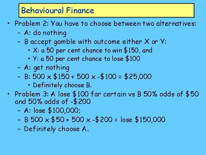
Behavioural Finance • Problem 2: You have to choose between two alternatives: – A: do nothing – B accept gamble with outcome either X or Y: • X: a 50 per cent chance to win $150, and • Y: a 50 per cent chance to lose $100. – What would you choose: option A or option B? – Would your choice change if your overall wealth were lower by $100? • Write your choice down: – A or B? – Would your choice change?

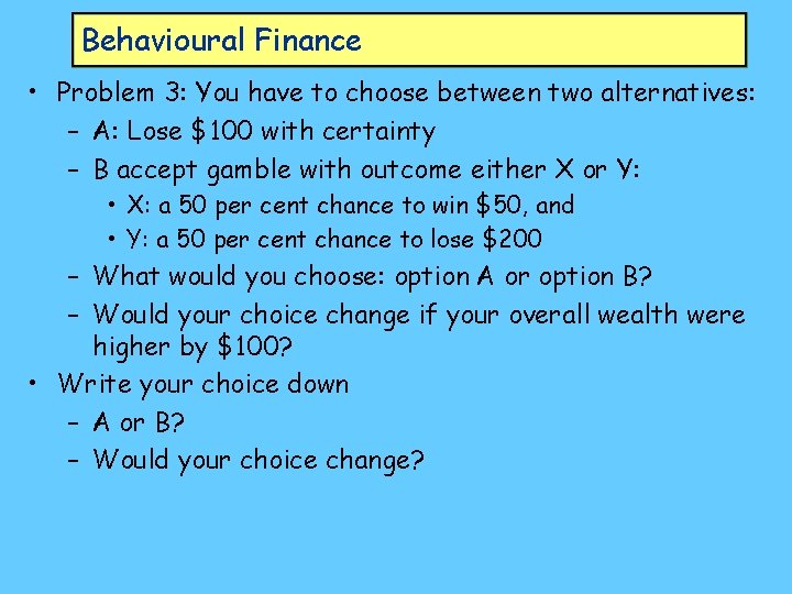
Behavioural Finance • Problem 3: You have to choose between two alternatives: – A: Lose $100 with certainty – B accept gamble with outcome either X or Y: • X: a 50 per cent chance to win $50, and • Y: a 50 per cent chance to lose $200 – What would you choose: option A or option B? – Would your choice change if your overall wealth were higher by $100? • Write your choice down – A or B? – Would your choice change?

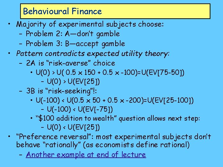
Behavioural Finance • Majority of experimental subjects choose: – Problem 2: A—don’t gamble – Problem 3: B—accept gamble • Pattern contradicts expected utility theory: – 2 A is “risk-averse” choice • U(0) > U( 0. 5 x 150 + 0. 5 x -100)=U(EV[75 -50]) – U(0) > U(EV[25]) – 3 B is “risk-seeking”!: • U(-100) < U(0. 5 x 50 + 0. 5 x -200)=U(EV[25 -100]) – U(-100) < U(EV[-75]) • “$100 addition to wealth” question allows next step: – U(0) < U(EV[25]) • “Preference reversal”: most experimental subjects don’t behave “rationally” (as economists define rational) – Another example at end of lecture

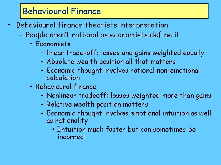
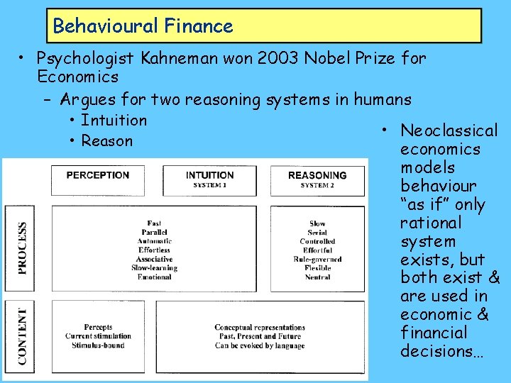
Behavioural Finance • Behavioural finance theorists interpretation – People aren’t rational as economists define it • Economists – linear trade-off: losses and gains weighted equally – Absolute wealth position all that matters – Economic thought involves rational non-emotional calculation • Behavioural finance – Nonlinear tradeoff: losses weighted more than gains – Relative wealth position matters – Economic thought involves emotional intuition as well as rationality • Intuition much faster but can sometimes be incorrect

Behavioural Finance • Psychologist Kahneman won 2003 Nobel Prize for Economics – Argues for two reasoning systems in humans • Intuition • Reason • Neoclassical economics models behaviour “as if” only rational system exists, but both exist & are used in economic & financial decisions…

Behavioural Finance • Intuitive, emotional, relative judgments lie behind standard choices by experimental subjects: – “the very abrupt switch from risk aversion to risk seeking could not plausibly be explained by a utility function for wealth. Preferences appeared to be determined by attitudes to gains and losses, defined relative to a reference point… We therefore proposed an alternative theory of risk, in which the carriers of utility are gains and losses—changes of wealth rather than states” (Kahneman Nobel Prize lecture: 1456) • In “prospect theory”, people react more to losses than gains: pain of loss weighted more heavily than pleasure of gain

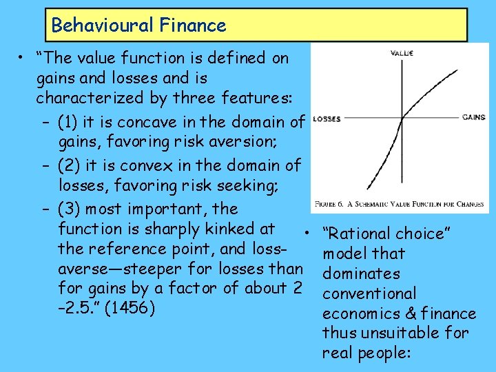
Behavioural Finance • “The value function is defined on gains and losses and is characterized by three features: – (1) it is concave in the domain of gains, favoring risk aversion; – (2) it is convex in the domain of losses, favoring risk seeking; – (3) most important, the function is sharply kinked at • the reference point, and lossaverse—steeper for losses than for gains by a factor of about 2 – 2. 5. ” (1456) “Rational choice” model that dominates conventional economics & finance thus unsuitable for real people:

Behavioural Finance • “The rational agent of economic theory would be described, in the language of the present treatment, as endowed with a single cognitive system that has the logical ability of a flawless System 2 and the low computing costs of System 1… • The [behavioural finance] model of the agent … has a different architecture The core ideas … are – the two-system structure, [intuition & reason] – the large role of System 1 [intuition] – and … extreme context-dependence… • The central characteristic of agents is not that they reason poorly but that they often act intuitively…” (1469) • Applied to stock market: Haugen’s “Inefficient Markets Hypothesis”

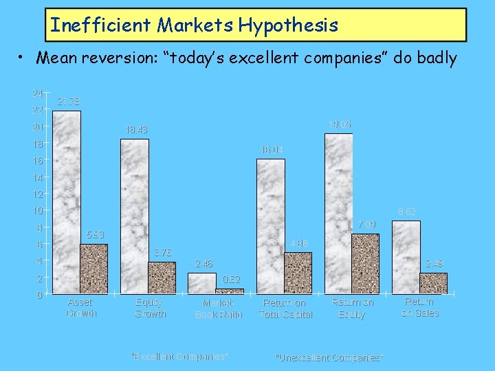
Inefficient Markets Hypothesis • Emphasises emotional component of investor decisionmaking – “Fad” (or Schumpeterian innovation) makes some industry sector or firm “growth stocks” • Valued above average Price to Book value (P/B) – Other unpopular “value” stocks ignored • Valued below average P/B ratio – Growth stocks inevitably disappoint – Value stocks often “surprise” • Repeated on scale of individual firms – Poor performing firm undervalued; good one overvalued – “Reversion to mean” causes “star” to disappoint, “dog” to outperform – Series of reports needed before trend spotted

Inefficient Markets Hypothesis • Institutional investors forced by need to match index to purchase broad portfolio – Non-institutional investors can profit by • Buying value stocks: Low P/B ratio & low earnings volatility • Timing entrance/exit from market • Many structural anomalies in stock market returns: – The “incredible January effect” • Rise of market almost every January – 95% of gains in December-April • Selective buy-in sell-out works • Some sample data from Bob Haugen (main proponent IMH) http: //www. bobhaugen. com/

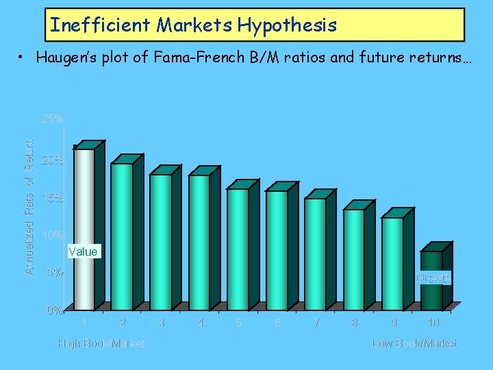
Inefficient Markets Hypothesis • Haugen’s plot of Fama-French B/M ratios and future returns… Annualized Rate of Return 25% 20% 15% 10% Value 5% 0% Growth 1 2 High Book/Market 3 4 5 6 7 8 9 10 Low Book/Market

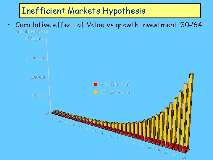
Inefficient Markets Hypothesis • Cumulative effect of Value vs growth investment ‘ 30 -’ 64 Cumulative Wealth $2, 000 $1, 500, 000 $1, 000 2. 47% Return 15. 18% Return $500, 000 $0 30 32 34 36 38 40 42 44 46 48 50 52 54 56 58 60 62 64

Inefficient Markets Hypothesis • Mean reversion: “today’s excellent companies” do badly 24 22 21. 78 20 19. 05 18. 43 18 16. 04 16 14 12 10 8 6 8. 62 7. 09 5. 93 3. 76 4 2. 46 2 0 4. 88 2. 49 0. 62 Asset Growth Equity Growth Market. Book Ratio "Excellent Companies" Return on Total Capital Return on Equity "Unexcellent Companies" Return on Sales

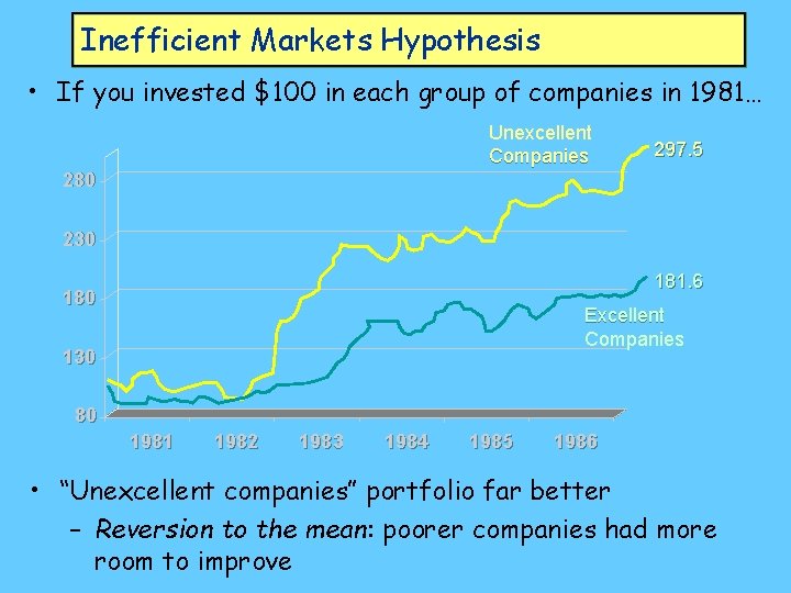
Inefficient Markets Hypothesis • If you invested $100 in each group of companies in 1981… Unexcellent Companies 297. 5 280 230 181. 6 180 Excellent Companies 130 80 1981 1982 1983 1984 1985 1986 • “Unexcellent companies” portfolio far better – Reversion to the mean: poorer companies had more room to improve

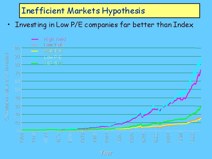
Inefficient Markets Hypothesis • Investing in Low P/E companies far better than Index High Yield Low Yield High P. E. Low P. E. S&P 500 90 80 70 60 50 40 30 20 Year 1996 1994 1992 1990 1988 1986 1984 1982 1980 1978 1976 1974 1972 0 1970 10 1968 Cumulative Value of $1 Invested 100

Behavioural Finance • Behavioural economics emphasises emotional, non-rational aspects of human decision making; • But 2 nd explanation of behavioural economics results: – Economics falsely applies risk theory to uncertainty – What economists call rational isn’t rational in uncertain world… • Expected value theory originally developed to interpret gambling: behaviour in risky games (roulette, cards, …) • Applied to economics after work on “Games & Economic Behaviour” by mathematician John von Neumann & economist Oskar Morgenstern • BUT: – von Neumann & Morgenstern used risk to build numerical theory of consumer choice…

Behavioural Finance • Mapping consumer preferences to arbitrary scale of “utils” using risk as guide to valuation: • Choice between: – one banana for certain or – gamble between no banana or 2 bananas • What odds of success needed before take gamble rather than sure thing? – Say consumer accepts 70% odds of success – Then 1 banana gives 70% of utility of 2 bananas – Set U(0)=0; U(1)=1 – Then U(1)/U(2) =0. 7: • U(2) = 1/0. 7 = 1. 43 • Numerical measure of utility intended to be complete replacement for indifference curve analysis:

Behavioural Finance • “It can be shown that under the conditions on which the indifference curve analysis is based very little extra effort is needed to reach a numerical utility. ” (von Neumann & Morgenstern 1944: 17) • “… if the preferences of the individual are not at all comparable, then the indifference curves do not exist. If the individual’s preferences are all comparable, then we can even obtain a (uniquely defined) numerical utility which renders the indifference curves superfluous. ” (1920) • Cautioned their concept of risk could not be subjective:

Behavioural Finance • “Probability has often been visualized as a subjective concept more or less in the nature of estimation. Since we propose to use it in constructing an individual, numerical estimation of utility, the above view of probability would not serve our purpose. The simplest procedure is, therefore, to insist upon the alternative, perfectly well founded interpretation of probability as frequency in long runs. ” (von Neumann & Morgenstern 1944: 19) • i. e. , risk of receiving banana had to mean average outcome of lots of gambles: – Banana a day for rest of your life; vs – 70% chance of 2 bananas vs zero for rest of your life – Reconsider first example this way:

Behavioural Finance • Problem 1: You have to choose between two alternatives: – A: 50% chance of $100 and 50% chance of nothing – B: 75% chance of $200 and 25% chance of -$100 – Whatever you choose will be repeated 1000 times • You’d have to be stupid to choose A over B: – A: Win $100 500 times + Nothing 500 times • Total winnings over 1000 games = $50, 000 – B: Win $200 750 times+ lose $100 250 times • Total winnings over 1000 games = $125, 000 • Ditto for other problem:

Behavioural Finance • Problem 2: You have to choose between two alternatives: – A: do nothing – B accept gamble with outcome either X or Y: • X: a 50 per cent chance to win $150, and • Y: a 50 per cent chance to lose $100 – A: get nothing – B: 500 x $150 + 500 x -$100 = $25, 000 • Definitely choose B. • Problem 3: A lose $100 for certain vs B 50% odds of $50 and 50% odds of -$200 – A: lose $100, 000; – B 500 x $50 + 500 x -$200 = lose $150, 000 – Definitely choose A.

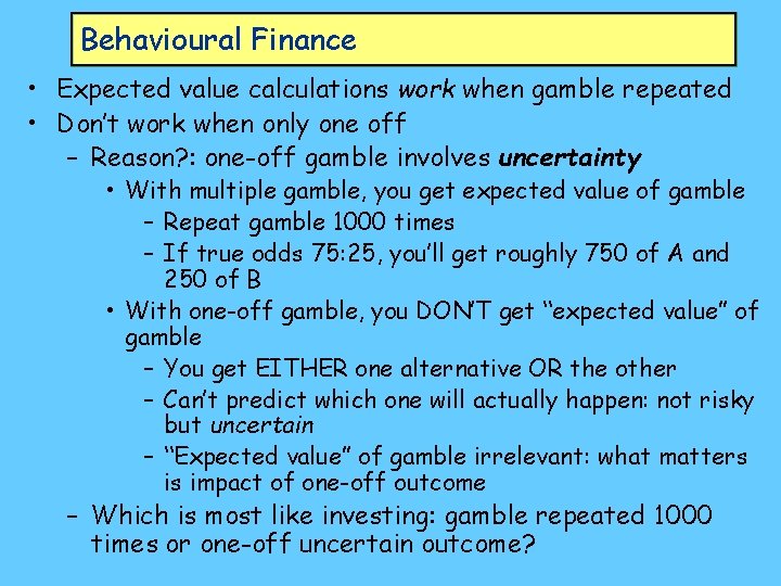
Behavioural Finance • Expected value calculations work when gamble repeated • Don’t work when only one off – Reason? : one-off gamble involves uncertainty • With multiple gamble, you get expected value of gamble – Repeat gamble 1000 times – If true odds 75: 25, you’ll get roughly 750 of A and 250 of B • With one-off gamble, you DON’T get “expected value” of gamble – You get EITHER one alternative OR the other – Can’t predict which one will actually happen: not risky but uncertain – “Expected value” of gamble irrelevant: what matters is impact of one-off outcome – Which is most like investing: gamble repeated 1000 times or one-off uncertain outcome?

Behavioural Finance • Investment decisions subject to uncertainty, not risk • Keynes emphatic about this in General Theory: – “factors … which determine the rate of investment … are most unreliable, since it is they which are influenced by our views of the future about which we know so little. ” • “no solid basis exists for a reasonable calculation” (154) • So … how do we decide how to invest? – we form conventions (see Lecture 9) – We try to minimise uncertainty • One method: “payback period” • Normally derided by economists

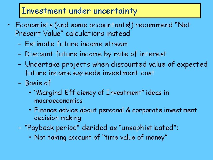
Investment under uncertainty • Economists (and some accountants!) recommend “Net Present Value” calculations instead – Estimate future income stream – Discount future income by rate of interest – Undertake projects when discounted value of expected future income exceeds investment cost – Basis of • “Marginal Efficiency of Investment” ideas in macroeconomics • Finance advice about personal & corporate investment decision making – “Payback period” derided as “unsophisticated”: • Not taking account of “time value of money”

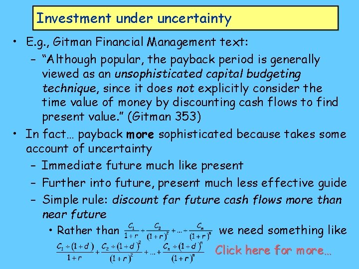
Investment under uncertainty • E. g. , Gitman Financial Management text: – “Although popular, the payback period is generally viewed as an unsophisticated capital budgeting technique, since it does not explicitly consider the time value of money by discounting cash flows to find present value. ” (Gitman 353) • In fact… payback more sophisticated because takes some account of uncertainty – Immediate future much like present – Further into future, present much less effective guide – Simple rule: discount far future cash flows more than near future we need something like • Rather than Click here for more…

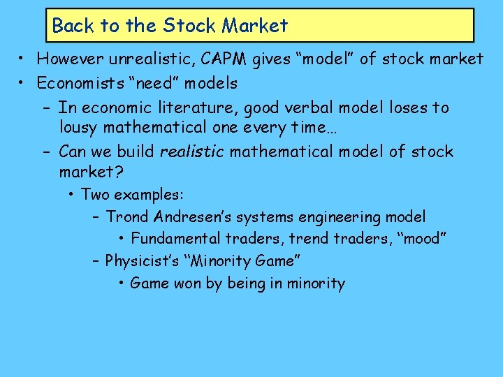
Back to the Stock Market • However unrealistic, CAPM gives “model” of stock market • Economists “need” models – In economic literature, good verbal model loses to lousy mathematical one every time… – Can we build realistic mathematical model of stock market? • Two examples: – Trond Andresen’s systems engineering model • Fundamental traders, trend traders, “mood” – Physicist’s “Minority Game” • Game won by being in minority

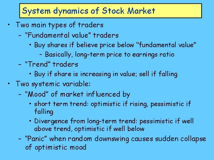
System dynamics of Stock Market • Two main types of traders – “Fundamental value” traders • Buy shares if believe price below “fundamental value” – Basically, long-term price to earnings ratio – “Trend” traders • Buy if share is increasing in value; sell if falling • Two systemic variable: – “Mood” of market influenced by • short term trend: optimistic if rising, pessimistic if falling • Divergence from long-term trend: pessimistic if well above trend, optimistic if well below – “Panic” when random downswing causes sudden collapse of optimistic mood

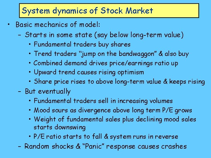
System dynamics of Stock Market • Basic mechanics of model: – Starts in some state (say below long-term value) • • • Fundamental traders buy shares Trend traders “jump on the bandwaggon” & also buy Combined demand drives price/earnings ratio up Upward trend causes rising optimism Share price rises to above long-term value & keeps rising – But eventually • Fundamental traders sell in increasing volumes • Mood sours as divergence above long term P/E grows • Weight of fundamental sales plus declining mood sales starts downswing • P/E ratio starts to fall & system runs in reverse – Random shocks & “Panic” response causes crashes

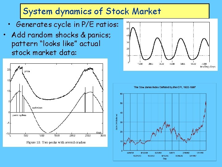
System dynamics of Stock Market • Generates cycle in P/E ratios: • Add random shocks & panics; pattern “looks like” actual stock market data:

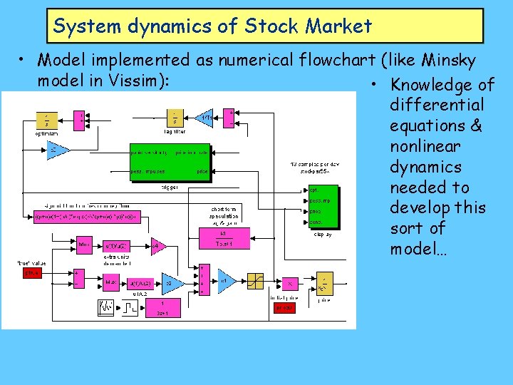
System dynamics of Stock Market • Model implemented as numerical flowchart (like Minsky model in Vissim): • Knowledge of differential equations & nonlinear dynamics needed to develop this sort of model…

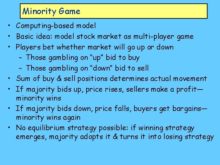
Minority Game • Computing-based model • Basic idea: model stock market as multi-player game • Players bet whether market will go up or down – Those gambling on “up” bid to buy – Those gambling on “down” bid to sell • Sum of buy & sell positions determines actual movement • If majority bids up, price rises, sellers make a profit— minority wins • If majority bids down, price falls, buyers get bargains— minority wins again • No equilibrium strategy possible: if winning strategy emerges, majority adopts it & turns it into losing strategy

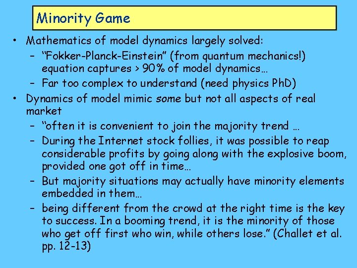
Minority Game • Mathematics of model dynamics largely solved: – “Fokker-Planck-Einstein” (from quantum mechanics!) equation captures > 90% of model dynamics… – Far too complex to understand (need physics Ph. D) • Dynamics of model mimic some but not all aspects of real market – “often it is convenient to join the majority trend … – During the Internet stock follies, it was possible to reap considerable profits by going along with the explosive boom, provided one got off in time… – But majority situations may actually have minority elements embedded in them… – being different from the crowd at the right time is the key to success. In a booming trend, it is the minority of those who get off first who win, while others lose. ” (Challet et al. pp. 12 -13)

Whew! Next week… • Overview of conventional trade theory • Final week: critique of comparative advantage & outline of “competitive advantage”

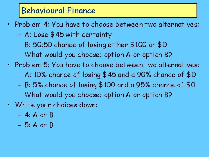
Behavioural Finance • Problem 4: You have to choose between two alternatives: – A: Lose $45 with certainty – B: 50 chance of losing either $100 or $0 – What would you choose: option A or option B? • Problem 5: You have to choose between two alternatives: – A: 10% chance of losing $45 and a 90% chance of $0 – B: 5% chance of losing $100 and a 95% chance of $0 – What would you choose: option A or option B? • Write your choices down: – 4: A or B – 5: A or B

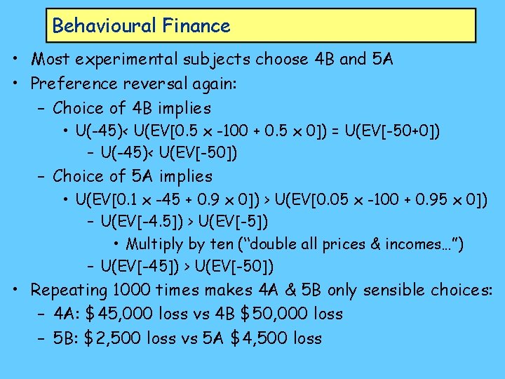
Behavioural Finance • Most experimental subjects choose 4 B and 5 A • Preference reversal again: – Choice of 4 B implies • U(-45)< U(EV[0. 5 x -100 + 0. 5 x 0]) = U(EV[-50+0]) – U(-45)< U(EV[-50]) – Choice of 5 A implies • U(EV[0. 1 x -45 + 0. 9 x 0]) > U(EV[0. 05 x -100 + 0. 95 x 0]) – U(EV[-4. 5]) > U(EV[-5]) • Multiply by ten (“double all prices & incomes…”) – U(EV[-45]) > U(EV[-50]) • Repeating 1000 times makes 4 A & 5 B only sensible choices: – 4 A: $45, 000 loss vs 4 B $50, 000 loss – 5 B: $2, 500 loss vs 5 A $4, 500 loss

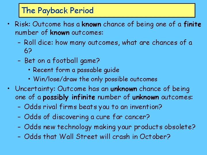
The Payback Period • Risk: Outcome has a known chance of being one of a finite number of known outcomes: – Roll dice: how many outcomes, what are chances of a 6? – Bet on a football game? • Recent form a passable guide • Win/lose/draw the only possible outcomes • Uncertainty: Outcome has an unknown chance of being one of a possibly infinite number of unknown outcomes: – Odds rival firms beats you to an invention? – Odds of discovering a cure for cancer? – Odds new technology making your products obsolete? – Odds that Wall Street will crash in October?

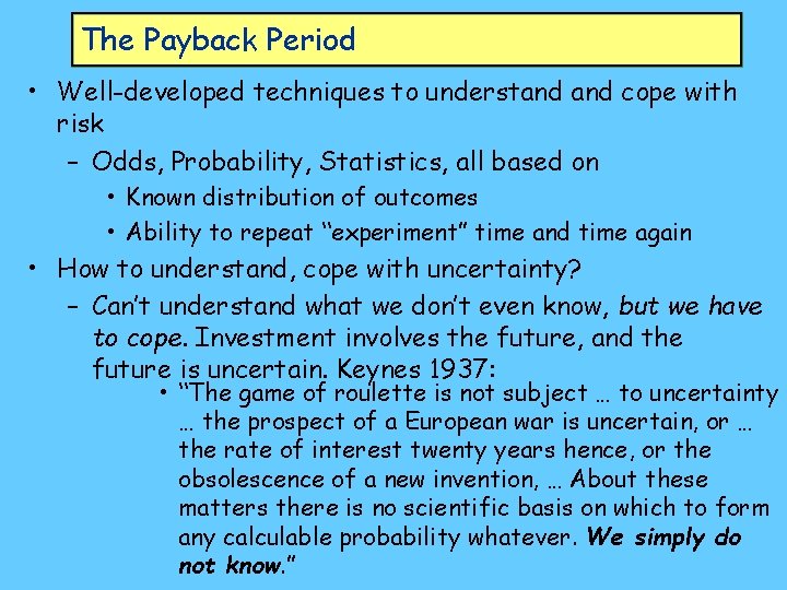
The Payback Period • Well-developed techniques to understand cope with risk – Odds, Probability, Statistics, all based on • Known distribution of outcomes • Ability to repeat “experiment” time and time again • How to understand, cope with uncertainty? – Can’t understand what we don’t even know, but we have to cope. Investment involves the future, and the future is uncertain. Keynes 1937: • “The game of roulette is not subject … to uncertainty … the prospect of a European war is uncertain, or … the rate of interest twenty years hence, or the obsolescence of a new invention, … About these matters there is no scientific basis on which to form any calculable probability whatever. We simply do not know. ”

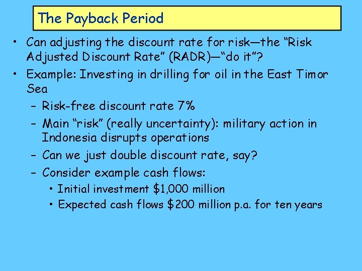
The Payback Period • Can adjusting the discount rate for risk—the “Risk Adjusted Discount Rate” (RADR)—“do it”? • Example: Investing in drilling for oil in the East Timor Sea – Risk-free discount rate 7% – Main “risk” (really uncertainty): military action in Indonesia disrupts operations – Can we just double discount rate, say? – Consider example cash flows: • Initial investment $1, 000 million • Expected cash flows $200 million p. a. for ten years

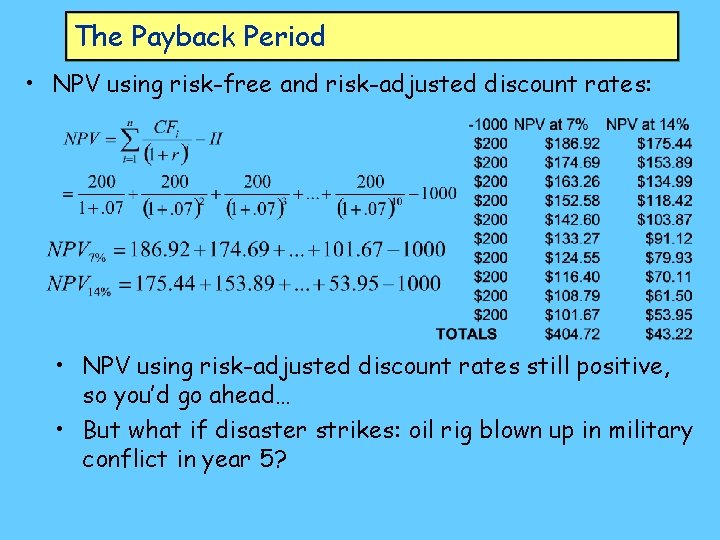
The Payback Period • NPV using risk-free and risk-adjusted discount rates: • NPV using risk-adjusted discount rates still positive, so you’d go ahead… • But what if disaster strikes: oil rig blown up in military conflict in year 5?

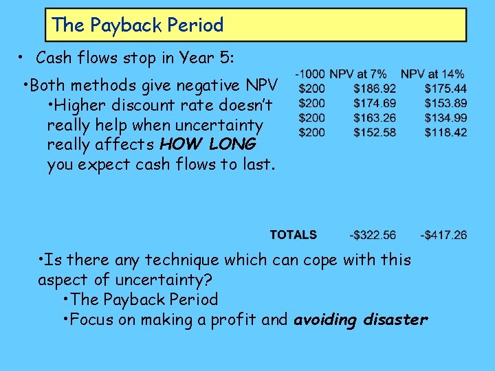
The Payback Period • Cash flows stop in Year 5: • Both methods give negative NPV • Higher discount rate doesn’t really help when uncertainty really affects HOW LONG you expect cash flows to last. • Is there any technique which can cope with this aspect of uncertainty? • The Payback Period • Focus on making a profit and avoiding disaster

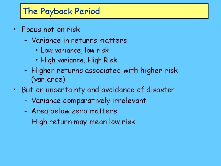
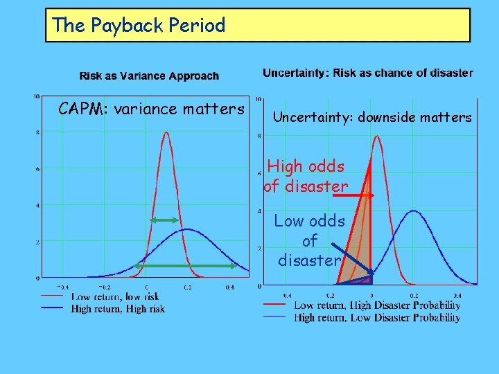
The Payback Period • Focus not on risk – Variance in returns matters • Low variance, low risk • High variance, High Risk – Higher returns associated with higher risk (variance) • But on uncertainty and avoidance of disaster – Variance comparatively irrelevant – Area below zero matters – High return may mean low risk

The Payback Period CAPM: variance matters Uncertainty: downside matters High odds of disaster Low odds of disaster

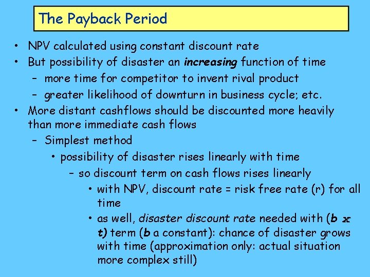
The Payback Period • NPV calculated using constant discount rate • But possibility of disaster an increasing function of time – more time for competitor to invent rival product – greater likelihood of downturn in business cycle; etc. • More distant cashflows should be discounted more heavily than more immediate cash flows – Simplest method • possibility of disaster rises linearly with time – so discount term on cash flows rises linearly • with NPV, discount rate = risk free rate (r) for all time • as well, disaster discount rate needed with (b x t) term (b a constant): chance of disaster grows with time (approximation only: actual situation more complex still)

The Payback Period • NPV formula in discrete form is Expected value Inflow in year i Discount rate • In continuous time form this is Cash flows as a function of time • If disaster strikes at time s, then the NPV of cash flows only will be • Since all cash flows after time s are zero (ignoring disaster related negatives—e. g. , Exxon Valdize cleanup costs)

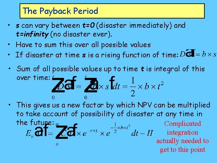
The Payback Period • s can vary between t=0 (disaster immediately) and t=infinity (no disaster ever). • Have to sum this over all possible values • If disaster at time s is a rising function of time: • Sum of all possible values up to time t is integral of this over time: • This gives us a new factor by which NPV can be multiplied to take account of possibility of disaster at any time in the future: Complicated integration actually needed to get to this point

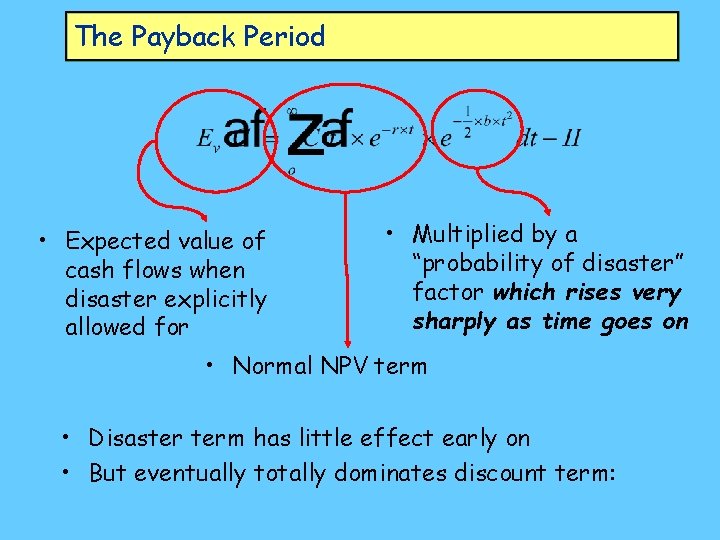
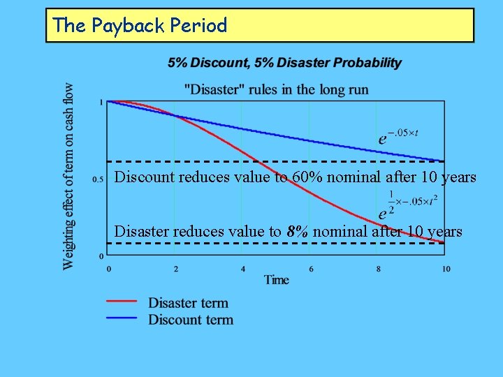
The Payback Period • Expected value of cash flows when disaster explicitly allowed for • Multiplied by a “probability of disaster” factor which rises very sharply as time goes on • Normal NPV term • Disaster term has little effect early on • But eventually totally dominates discount term:

The Payback Period Discount reduces value to 60% nominal after 10 years Disaster reduces value to 8% nominal after 10 years

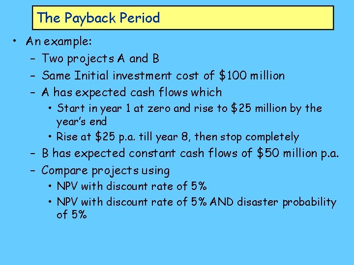
The Payback Period • An example: – Two projects A and B – Same Initial investment cost of $100 million – A has expected cash flows which • Start in year 1 at zero and rise to $25 million by the year’s end • Rise at $25 p. a. till year 8, then stop completely – B has expected constant cash flows of $50 million p. a. – Compare projects using • NPV with discount rate of 5% AND disaster probability of 5%

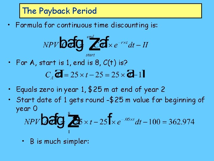
The Payback Period • Formula for continuous time discounting is: • For A, start is 1, end is 8, C(t) is? • Equals zero in year 1, $25 m at end of year 2 • Start date of 1 gets round -$25 m value for beginning of year 0 • B is much simpler:

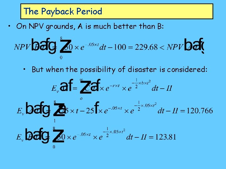
The Payback Period • On NPV grounds, A is much better than B: • But when the possibility of disaster is considered:

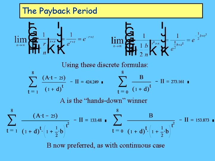
The Payback Period • Values drastically lower than NPV levels – strong impact of uncertainty • Priority reversed – more immediate cash flows of B preferred to higher but delayed cash flows of A • Almost the same result for less accurate discrete formulas: • As with discount, discrete disaster term approximates continuous term:

The Payback Period Using these discrete formulas: A is the “hands-down” winner B now preferred, as with continuous case

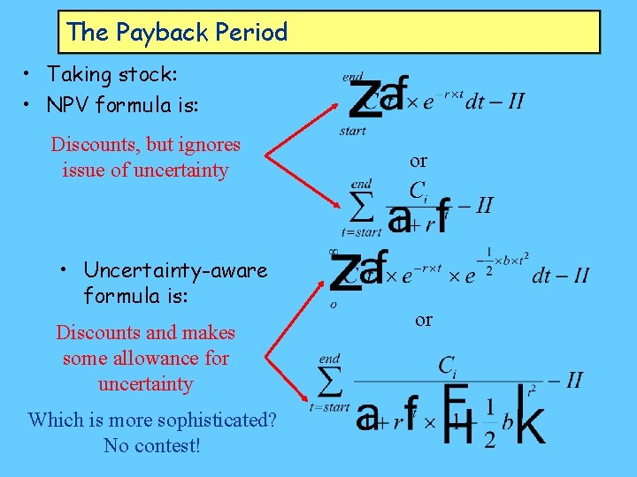
The Payback Period • Taking stock: • NPV formula is: Discounts, but ignores issue of uncertainty • Uncertainty-aware formula is: Discounts and makes some allowance for uncertainty Which is more sophisticated? No contest! or or

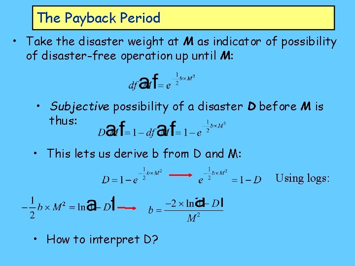
The Payback Period • Do businessmen use anything so complicated? – Of course not • (but might expect their financial advisers to do so!) • Is there anything businesses commonly use that approximates to this? – Yes: The Payback Period • Payback period – Puts maximum time M allowed for project to cover initial costs – Ranks projects within time limit on basis of expected revenues • We can relate M to previous formulas and idea of probability of disaster D striking before payback period M:

The Payback Period • Take the disaster weight at M as indicator of possibility of disaster-free operation up until M: • Subjective possibility of a disaster D before M is thus: • This lets us derive b from D and M: Using logs: • How to interpret D?

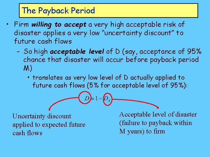
The Payback Period • Firm willing to accept a very high acceptable risk of disaster applies a very low “uncertainty discount” to future cash flows – So high acceptable level of D (say, acceptance of 95% chance that disaster will occur before payback period M) • translates as very low level of D actually applied to future cash flows (5% for acceptable level of 95%): Uncertainty discount applied to expected future cash flows Acceptable level of disaster (failure to payback within M years) to firm

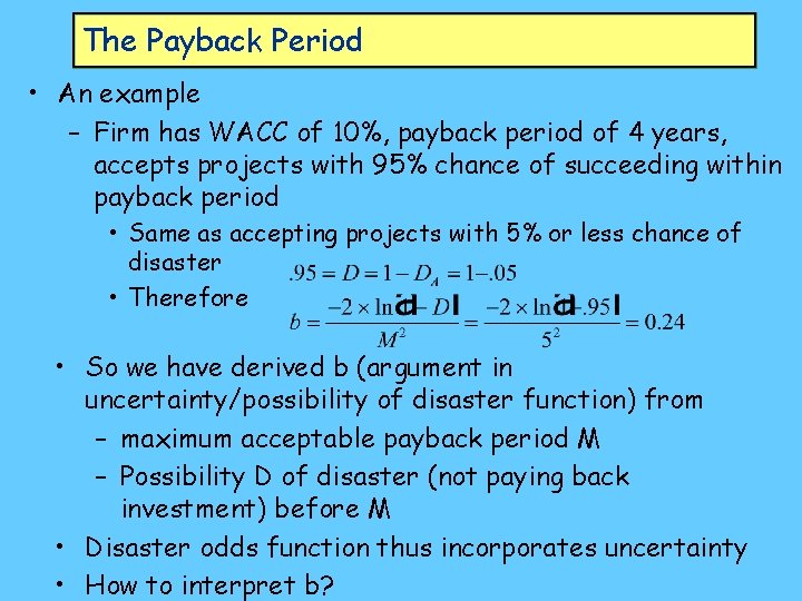
The Payback Period • An example – Firm has WACC of 10%, payback period of 4 years, accepts projects with 95% chance of succeeding within payback period • Same as accepting projects with 5% or less chance of disaster • Therefore • So we have derived b (argument in uncertainty/possibility of disaster function) from – maximum acceptable payback period M – Possibility D of disaster (not paying back investment) before M • Disaster odds function thus incorporates uncertainty • How to interpret b?

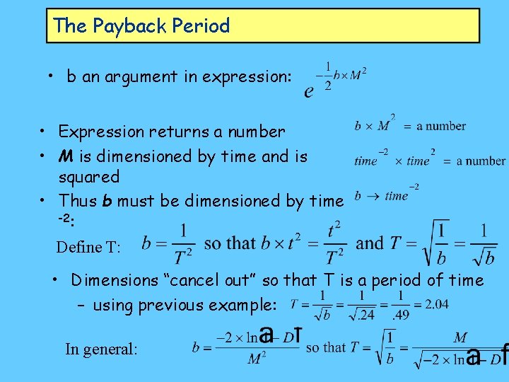
The Payback Period • b an argument in expression: • Expression returns a number • M is dimensioned by time and is squared • Thus b must be dimensioned by time -2: Define T: • Dimensions “cancel out” so that T is a period of time – using previous example: In general:

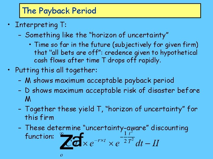
The Payback Period • Interpreting T: – Something like the “horizon of uncertainty” • Time so far in the future (subjectively for given firm) that “all bets are off”: credence given to hypothetical cash flows after time T drops off rapidly. • Putting this all together: – M shows maximum acceptable payback period – D shows maximum acceptable risk of disaster before M – Together these yield T, “horizon of uncertainty” for this firm – These determine “uncertainty-aware” discounting function:

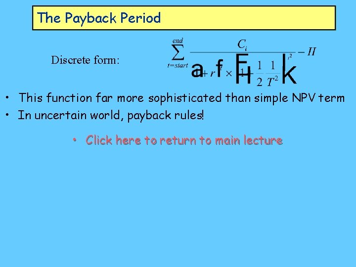
The Payback Period Discrete form: • This function far more sophisticated than simple NPV term • In uncertain world, payback rules! • Click here to return to main lecture