Managerial Economics Lecture Ten Standard theory of finance

Managerial Economics Lecture Ten: Standard theory of finance

Recap • Minsky’s “Financial Instability Hypothesis” – Finance-driven cyclical behavior

“Modern” Finance? • “Modern Finance Theory” has many components: – Sharpe’s “Capital Asset Pricing Model” (CAPM) – Modigliani-Miller’s “Dividend Irrelevance Theorem” – Markowitz’s risk-averse portfolio optimisation model – Arbitrage Pricing Theory (APT) • “Modern” as compared to pre-1950 theories that emphasised behaviour of investors as explanation of stock prices, value investing, etc. – Initially appeared to explain what “old finance” could not – But 50 years on… • Foundation is Sharpe’s CAPM:

The Capital Assets Pricing Model • How to “predict the behaviour of capital markets”? • Extend theories of investment under certainty. . . – to investment under conditions of risk • Based on neoclassical utility theory • Investor maximises utility subject to constraints • Utility: – Positive function of expected return ER – Negative function of risk (standard deviation) s. R • Constraints are available spectrum of investment opportunities

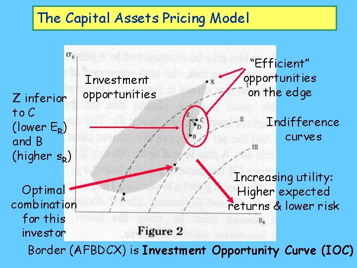
The Capital Assets Pricing Model Z inferior to C (lower ER) and B (higher s. R) Investment opportunities “Efficient” opportunities on the edge Indifference curves Increasing utility: Higher expected returns & lower risk Optimal combination for this investor Border (AFBDCX) is Investment Opportunity Curve (IOC)

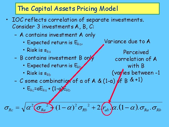
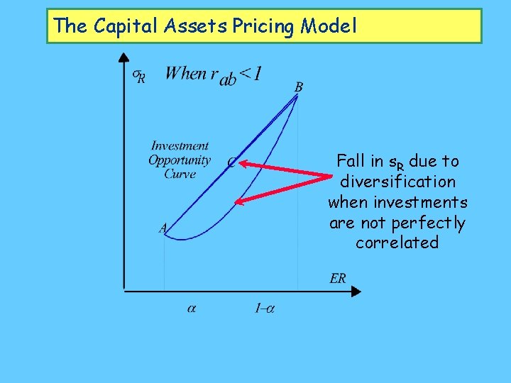
The Capital Assets Pricing Model • IOC reflects correlation of separate investments. Consider 3 investments A, B, C: – A contains investment A only Variance due to A • Expected return is ERa, • Risk is s. Ra Perceived – B contains investment B only correlation of A • Expected return is ERb, with B (varies between -1 • Risk is s. Rb – C some combination of a of A & (1 -a) of B & +1) • ERc=a. ERa + (1 -a)ERb

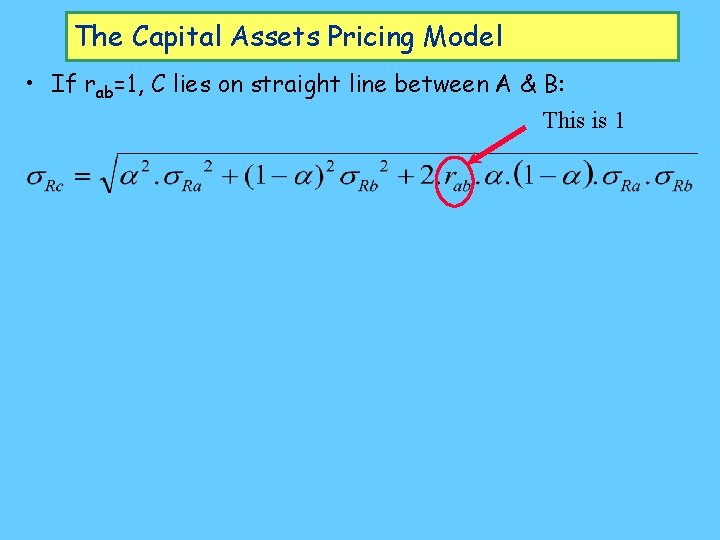
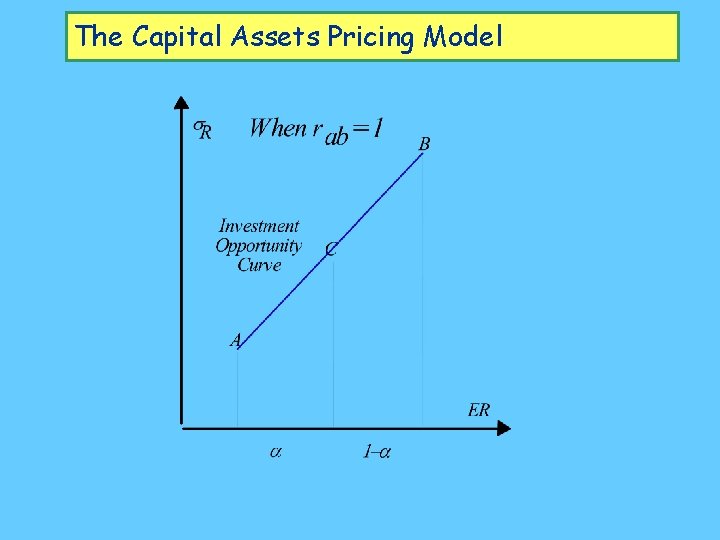
The Capital Assets Pricing Model • If rab=1, C lies on straight line between A & B: This is 1

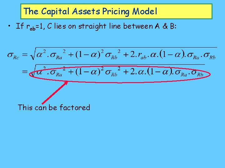
The Capital Assets Pricing Model • If rab=1, C lies on straight line between A & B: This can be factored

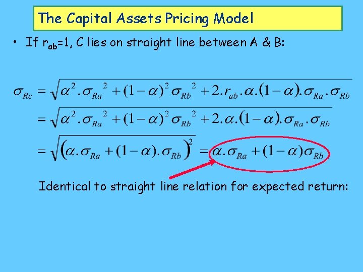
The Capital Assets Pricing Model • If rab=1, C lies on straight line between A & B: Identical to straight line relation for expected return:

The Capital Assets Pricing Model

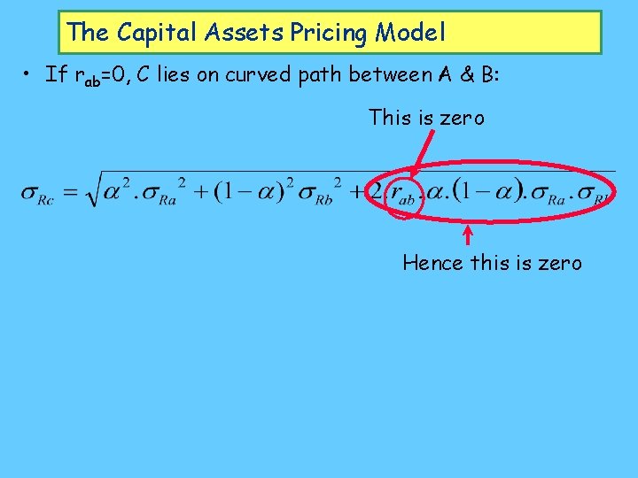
The Capital Assets Pricing Model • If rab=0, C lies on curved path between A & B: This is zero Hence this is zero

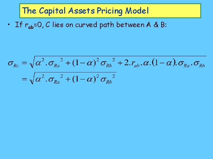
The Capital Assets Pricing Model • If rab=0, C lies on curved path between A & B:

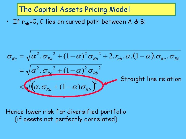
The Capital Assets Pricing Model • If rab=0, C lies on curved path between A & B: Straight line relation Hence lower risk for diversified portfolio (if assets not perfectly correlated)

The Capital Assets Pricing Model Fall in s. R due to diversification when investments are not perfectly correlated

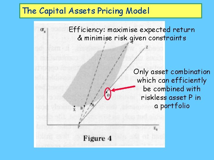
The Capital Assets Pricing Model • Sharpe assumes riskless asset P with ERP=pure interest rate, s. RP=0. • Investor can form portfolio of P with any other combination of assets • One asset combination will initially dominate all others:

The Capital Assets Pricing Model Efficiency: maximise expected return & minimise risk given constraints Only asset combination which can efficiently be combined with riskless asset P in a portfolio

The Capital Assets Pricing Model • Assume limitless borrowing/lending at riskless interest rate = return on asset P • Investor can move to anywhere along Pf. Z line by borrowing/lending • Problem: – P the same for all investors (“simplifying assumption”) – But investor perceptions of expected return, risk, investment correlation will differ • Solution: – assume “homogeneity of investor expectations” – utterly unrealistic assumption, as is assumption of limitless borrowing by all borrowers at riskless interest rate. So. . .

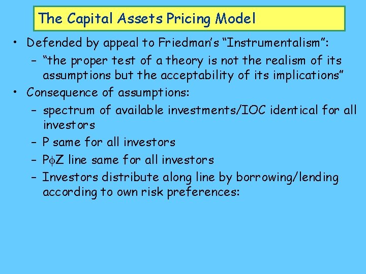
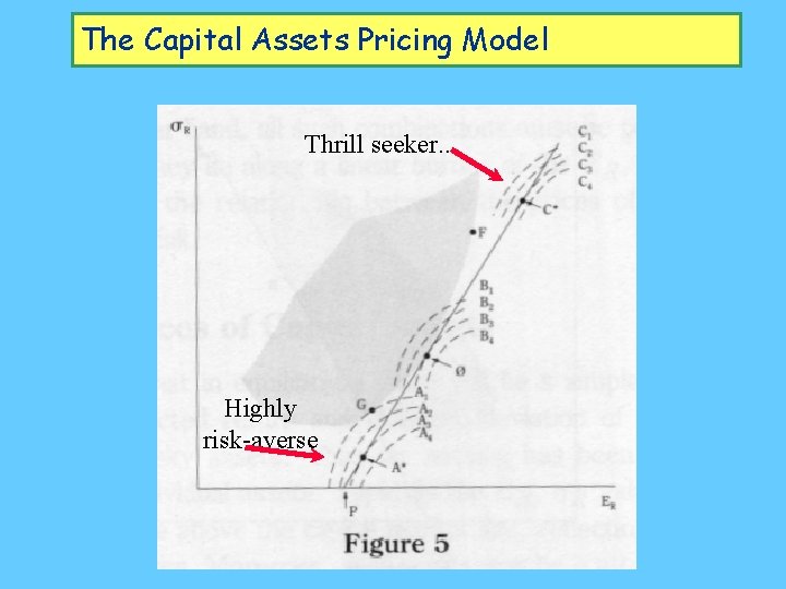
The Capital Assets Pricing Model • Defended by appeal to Friedman’s “Instrumentalism”: – “the proper test of a theory is not the realism of its assumptions but the acceptability of its implications” • Consequence of assumptions: – spectrum of available investments/IOC identical for all investors – P same for all investors – Pf. Z line same for all investors – Investors distribute along line by borrowing/lending according to own risk preferences:

The Capital Assets Pricing Model Thrill seeker. . . Highly risk-averse

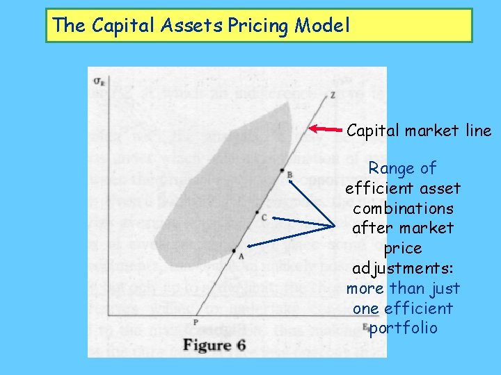
The Capital Assets Pricing Model • Next, the (perfect) market mechanism – Price of assets in f will rise – Price of assets not in f will fall – Price changes shift expected returns – Causes new pattern of efficient investments aligned with Pf. Z line:

The Capital Assets Pricing Model Capital market line Range of efficient asset combinations after market price adjustments: more than just one efficient portfolio

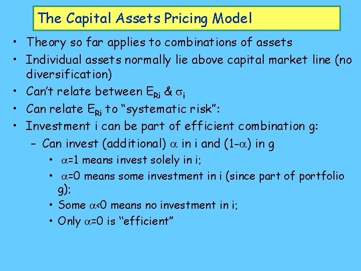
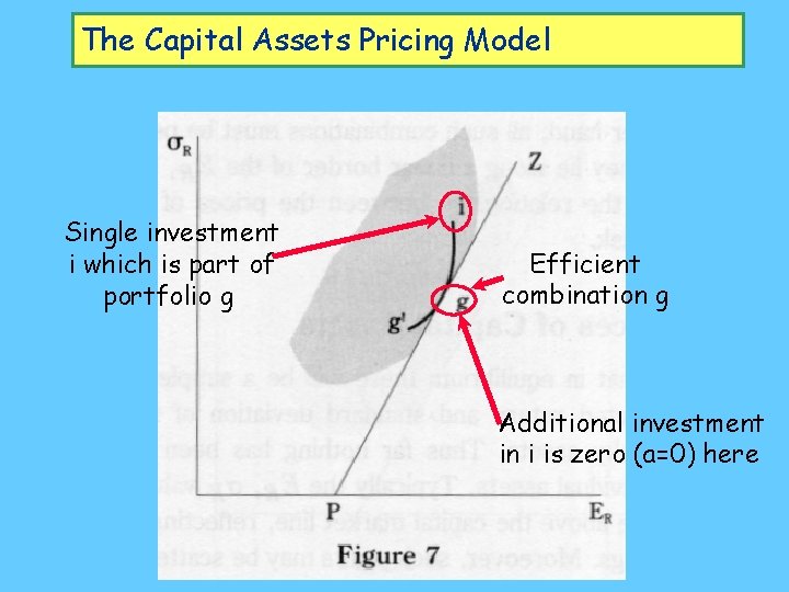
The Capital Assets Pricing Model • Theory so far applies to combinations of assets • Individual assets normally lie above capital market line (no diversification) • Can’t relate between ERi & si • Can relate ERi to “systematic risk”: • Investment i can be part of efficient combination g: – Can invest (additional) a in i and (1 -a) in g • a=1 means invest solely in i; • a=0 means some investment in i (since part of portfolio g); • Some a<0 means no investment in i; • Only a=0 is “efficient”

The Capital Assets Pricing Model Single investment i which is part of portfolio g Efficient combination g Additional investment in i is zero (a=0) here

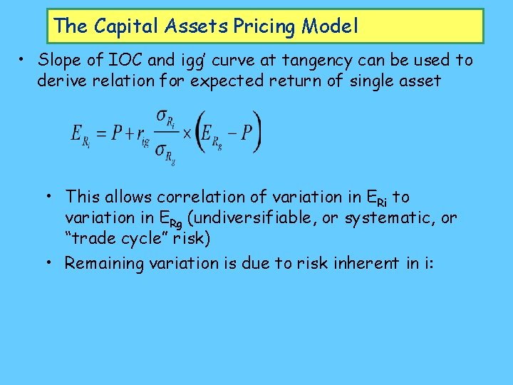
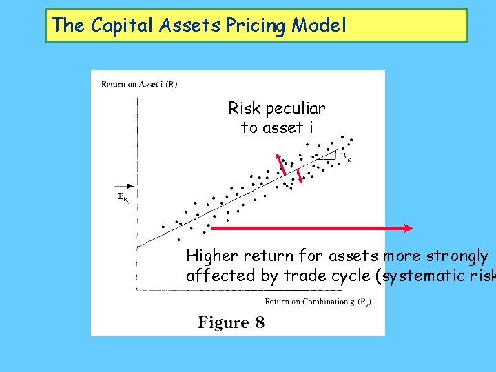
The Capital Assets Pricing Model • Slope of IOC and igg’ curve at tangency can be used to derive relation for expected return of single asset • This allows correlation of variation in ERi to variation in ERg (undiversifiable, or systematic, or “trade cycle” risk) • Remaining variation is due to risk inherent in i:

The Capital Assets Pricing Model Risk peculiar to asset i Higher return for assets more strongly affected by trade cycle (systematic risk

The Capital Assets Pricing Model • Efficient portfolio enables investor to minimise asset specific risk • Systematic risk (risk inherent in efficient portfolio) can’t be diversified against • Hence market prices adjust to degree of responsiveness of investments to trade cycle: – “Assets which are unaffected by changes in economic activity will return the pure interest rate; those which move with economic activity will promise appropriately higher expected rates of return. ” [OREF II]

The Capital Assets Pricing Model • Crux/basis of model: markets efficiently value investments on basis of expected returns/risk tradeoff • Modigliani-Miller extend model to argue valuation of firms independent of debt structure (see OREF II) • Combination: the “efficient markets hypothesis” • Focus on portfolio allocation across investments at a point in time, rather than trend of value over time • Argues investors focus on “fundamentals”: – Expected return – Risk • So long as assumptions are defensible…

The Capital Assets Pricing Model • “In order to derive conditions for equilibrium in the capital market we invoke two assumptions. First, we assume a common pure rate of interest, with all investors able to borrow or lend funds on equal terms. Second, we assume homogeneity of investor expectations: investors are assumed to agree on the prospects of various investments–the expected values, standard deviations and correlation coefficients described in Part II. Needless to say, these are highly restrictive and undoubtedly unrealistic assumptions. • However, since the proper test of a theory is not the realism of its assumptions but the acceptability of its implications, and since these assumptions imply equilibrium conditions which form a major part of classical financial doctrine, it is far from clear that this formulation should be rejected–especially in view of the dearth of alternative models leading to similar results. ” • Sharpe later admits to qualms…

The CAPM: Reservations • “People often hold passionately to beliefs that are far from universal. The seller of a share of IBM stock may be convinced that it is worth considerably less than the sales price. The buyer may be convinced that it is worth considerably more. ” (Sharpe 1970) • However, if we try to be more realistic: – “The consequence of accommodating such aspects of reality are likely to be disastrous in terms of the usefulness of the resulting theory. . . The capital market line no longer exists. Instead, there is a capital market curve–linear over some ranges, perhaps, but becoming flatter as [risk] increases over other ranges. Moreover, there is no single optimal combination of risky securities; the preferred combination depends upon the investors’ preferences. . . The demise of the capital market line is followed immediately by that of the security market line. The theory is in a shambles. ” (Sharpe 1970 emphasis added)

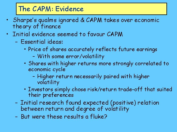
The CAPM: Evidence • Sharpe’s qualms ignored & CAPM takes over economic theory of finance • Initial evidence seemed to favour CAPM – Essential ideas: • Price of shares accurately reflects future earnings – With some error/volatility • Shares with higher returns more strongly correlated to economic cycle – Higher return necessarily paired with higher volatility • Investors simply chose risk/return trade-off that suited their preferences – Initial research found expected (positive) relation between return and degree of volatility – But were these results a fluke?

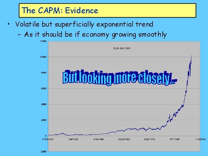
The CAPM: Evidence • Volatile but superficially exponential trend – As it should be if economy growing smoothly

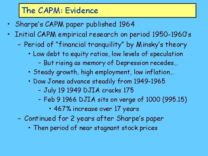
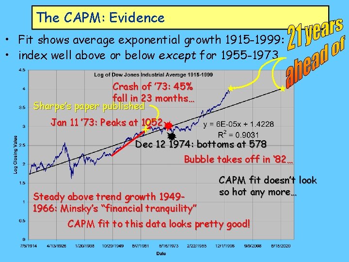
The CAPM: Evidence • Sharpe’s CAPM paper published 1964 • Initial CAPM empirical research on period 1950 -1960’s – Period of “financial tranquility” by Minsky’s theory • Low debt to equity ratios, low levels of speculation – But rising as memory of Depression recedes… • Steady growth, high employment, low inflation… • Dow Jones advance steadily from 1949 -1965 – July 19 1949 DJIA cracks 175 – Feb 9 1966 DJIA sits on verge of 1000 (995. 15) • 467% increase over 17 years – Continued for 2 years after Sharpe’s paper • Then period of near stagnant stock prices

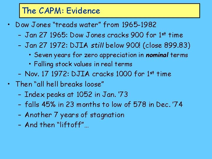
The CAPM: Evidence • Dow Jones “treads water” from 1965 -1982 – Jan 27 1965: Dow Jones cracks 900 for 1 st time – Jan 27 1972: DJIA still below 900! (close 899. 83) • Seven years for zero appreciation in nominal terms • Falling stock values in real terms – Nov. 17 1972: DJIA cracks 1000 for 1 st time • Then “all hell breaks loose” – Index peaks at 1052 in Jan. ‘ 73 – falls 45% in 23 months to low of 578 in Dec. ’ 74 – Another 7 years of stagnation – And then “liftoff”…

The CAPM: Evidence • Fit shows average exponential growth 1915 -1999: • index well above or below except for 1955 -1973 Crash of ’ 73: 45% fall in 23 months… Sharpe’s paper published Jan 11 ’ 73: Peaks at 1052 Dec 12 1974: bottoms at 578 Bubble takes off in ‘ 82… Steady above trend growth 19491966: Minsky’s “financial tranquility” CAPM fit doesn’t look so hot any more… CAPM fit to this data looks pretty good!

An aside: what caused ’ 73 crash? • Many blame OPEC Oil Embargo for economic downturn • October 17, 1973: OPEC bans export of oil to countries that supported Israel in 1973 Arab-Israeli War • Oil price rises 4 -fold from US$2. 50 to $10 a barrel • BUT embargo occurred 9 months after market peak • Quarterly GDP growth fell from 10. 1% in Q 1 1973 to 1. 6% in Q 3 ‘ 73 before embargo • Market already down 8% by October 17 to 963 • Rose in immediate aftermath to embargo • Real acceleration of crash occurred with Franklin National Bank of New York crisis from May-October 1974 • May 1 854; Dec 12 578: 32% fall in 7 months • Minsky’s “financial fragility” more important • OPEC-inspired inflation may have made crisis less severe: reduction of real debt burden

The CAPM: Evidence • By mid-1990 s, clear CAPM and reality weren’t related – “The Dow. . . stood at around 3, 600 in early 1994. – By 1999, it had passed 11, 000, more than tripling in five years. . . – However, over the same period, basic economic indicators did not come close to tripling. – U. S. … gross domestic product rose less than 30%, and almost half of this increase was due to inflation. – Corporate profits rose less than 60%, and that from a temporary recession-depressed base. – Viewed in the light of these figures, the stock price increase appears unwarranted and, certainly by historical standards, unlikely to persist…” (Schiller: 4)

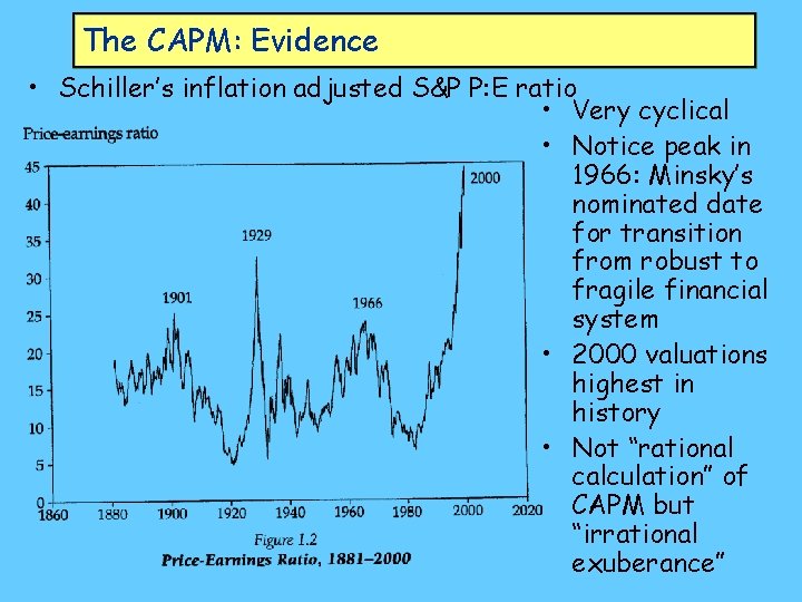
The CAPM: Evidence • Schiller’s inflation adjusted S&P P: E ratio • Very cyclical • Notice peak in 1966: Minsky’s nominated date for transition from robust to fragile financial system • 2000 valuations highest in history • Not “rational calculation” of CAPM but “irrational exuberance”

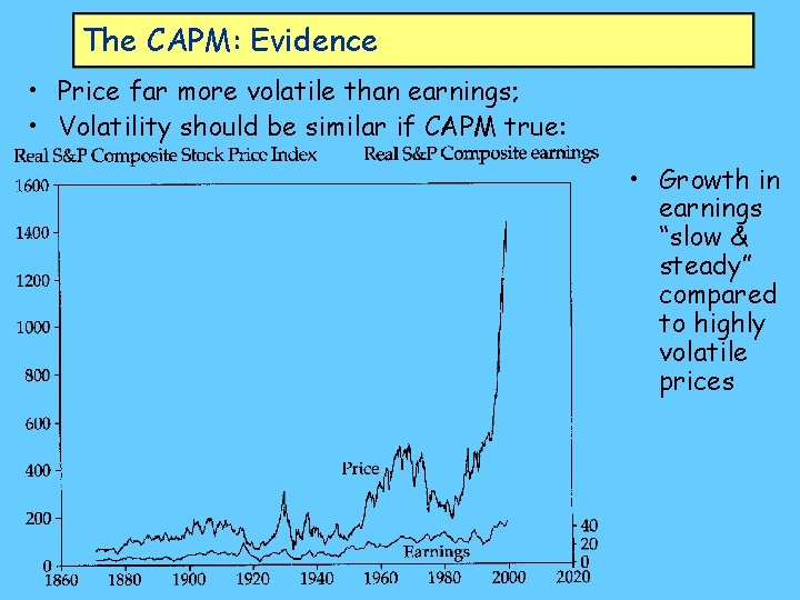
The CAPM: Evidence • Price far more volatile than earnings; • Volatility should be similar if CAPM true: • Growth in earnings “slow & steady” compared to highly volatile prices

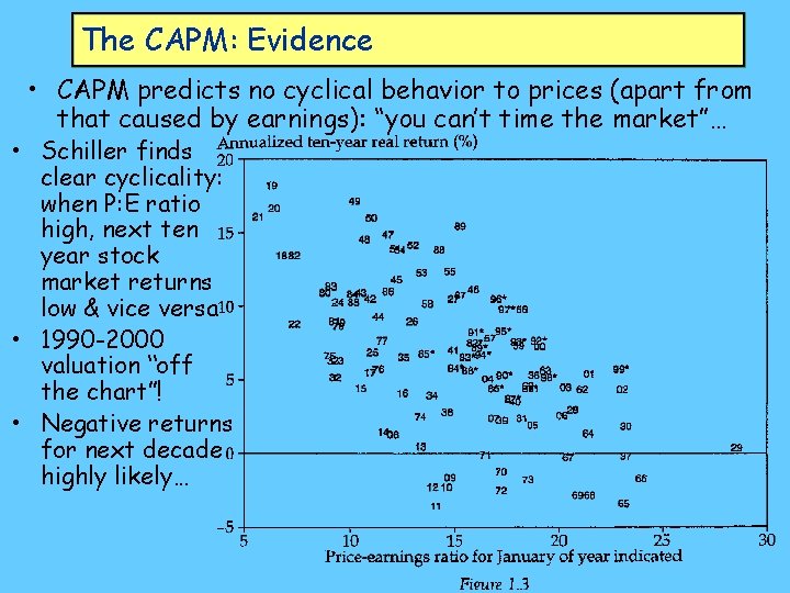
The CAPM: Evidence • CAPM predicts no cyclical behavior to prices (apart from that caused by earnings): “you can’t time the market”… • Schiller finds clear cyclicality: when P: E ratio high, next ten year stock market returns low & vice versa • 1990 -2000 valuation “off the chart”! • Negative returns for next decade highly likely…

The CAPM: Evidence • “The relation between price-earnings ratios and subsequent returns appears to be moderately strong. . . • longterm investors who can commit their money to an investment for ten full years do well when prices were low relative to earnings at the beginning of the ten years and do poorly when prices were high at the beginning of the ten years. • Long-term investors would be well advised, individually, to stay mostly out of the market when it is high, as it is today, and get into the market when it is low. ” (12) • Critics of CAPM thus dismiss it—but even its one-time champions do too – Fama & French

The CAPM: Evidence According to Fama 1969 • Evidence supports the CAPM – “This paper reviews theoretical and empirical literature on the efficient markets model… We shall conclude that, with but a few exceptions, the efficient markets model stands up well. ” (383) • Assumptions unrealistic but that doesn’t matter: – “the results of tests based on this assumption depend to some extent on its validity as well as on the efficiency of the market. But some such assumption is the unavoidable price one must pay to give theory of efficient markets empirical content. ” (384)

The CAPM: Evidence According to Fama 1969 • CAPM good guide to market behaviour – “For the purposes of most investors the efficient markets model seems a good first (and second) approximation to reality. ” (416) • Results conclusive – “In short, the evidence in support of the efficient markets model is extensive, and (somewhat uniquely in economics) contradictory evidence is sparse. ” (416) • Just one anomaly admitted to – Large movements one day often followed by large movements the next—“volatility clustering”…

The CAPM: Evidence According to Fama 1969 • “one departure from the pure independence assumption of the random walk model has been noted … large daily price changes tend to be followed by large daily changes. The signs of the successor changes are apparently random, however, which indicates that the phenomenon represents a denial of the random walk model but not of the market efficiency hypothesis… But since the evidence indicates that the price changes on days follow ing the initial large change are random in sign, the initial large change at least represents an unbiased adjustment to the ultimate price effects of the information, and this is sufficient for the expected return efficient markets model. ” (396) • 35 years later, picture somewhat different…

The CAPM: Evidence According to Fama 2004 • “The attraction of the CAPM is that it offers powerful and intuitively pleasing predictions about how to measure risk and the relation between expected return and risk. • Unfortunately, the empirical record of the model is poor—poor enough to invalidate the way it is used in applications. • The CAPM's empirical problems may reflect theoretical failings, the result of many simplifying assumptions… • In the end, we argue that whether the model's problems reflect weaknesses in theory or in its empirical implementation, the failure of the CAPM in empirical tests implies that most applications of the model are invalid. ” (Fama & French 2004: 25)

The CAPM: Evidence According to F&F 2004 • Clearly admits assumptions dangerously unrealistic: – “The first assumption is complete agreement given market clearing asset prices at t-1, investors agree on the joint distribution of asset returns from t-1 to t. And this distribution is the true one—that is, it is the distribution from which the returns we use to test the model are drawn. The second assumption is that there is borrowing and lending at a risk free rate, which is the same for all investors and does not depend on the amount borrowed or lent. ” (26) • Bold emphasis: model assumes all investors effectively know the future • Assumptions, which once “didn’t matter” (see Sharpe earlier) are now crucial…

The CAPM: Evidence According to F&F 2004 • “The assumption that short selling is unrestricted is as unrealistic as unrestricted risk-free borrowing and lending… But when there is no short selling of risky assets and no risk-free asset, the algebra of portfolio efficiency says that portfolios made up of efficient portfolios are not typically efficient. This means that the market portfolio, which is a portfolio of the efficient portfolios chosen by investors, is not typically efficient. And the CAPM relation between expected return and market beta is lost. ” (32) • Still some hope that, despite lack of realism, data might save the model…

The CAPM: Evidence According to F&F 2004 – “The efficiency of the market portfolio is based on many unrealistic assumptions, including complete agreement and either unrestricted risk-free borrowing and lending or unrestricted short selling of risky assets. But all interesting models involve unrealistic simplifications, which is why they must be tested against data. ” (32) • Unfortunately, no such luck… – 40 years of data strongly contradict all versions of CAPM • Returns not related to betas • Other variables (book to market ratios etc. ) matter • Linear regressions on data differ strongly from risk free rate (intercept) & beta (slope) calculations from CAPM

The CAPM: Evidence According to F&F 2004 • Tests of the CAPM are based on three implications… – “First, expected returns on all assets are linearly related to their betas, and no other variable has marginal explanatory power. – Second, the beta premium is positive, meaning that the expected return on the market portfolio exceeds the expected return on assets whose returns are uncorrelated with the market return. – Third, … assets uncorrelated with the market have expected returns equal to the risk-free interest rate, and the beta premium is the expected market return minus the risk-free rate. ” (32)

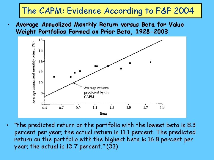
The CAPM: Evidence According to F&F 2004 • “There is a positive relation between beta and average return, but it is too "flat. " … the Sharpe-Lintner model predicts that – the intercept is the risk free rate and – the coefficient on beta is the expected market return in excess of the risk-free rate, E(RM) - R. – The regressions consistently find that the intercept is greater than the average risk-free rate…, and the coefficient on beta is less than the average excess market return” (32)

The CAPM: Evidence According to F&F 2004 • Average Annualized Monthly Return versus Beta for Value Weight Portfolios Formed on Prior Beta, 1928 -2003 • “the predicted return on the portfolio with the lowest beta is 8. 3 percent per year; the actual return is 11. 1 percent. The predicted return on the portfolio with the highest beta is 16. 8 percent per year; the actual is 13. 7 percent. ” (33)

The CAPM: Evidence According to F&F 2004 • The hypothesis that market betas completely explain expected returns … – Starting in the late 1970 s… evidence mounts that much of the variation in expected return is unrelated to market beta…” (34) – Fama and French (1992) update and synthesize the evidence on the empirical failures of the CAPM… they confirm that size, earnings-price, debt equity and book -to-market ratios add to the explanation of expected stock returns provided by market beta. ” (36) – Best example of failure of CAPM as guide to building investment portfolios: Book to Market (B/M) ratios provide far better guide than Beta…

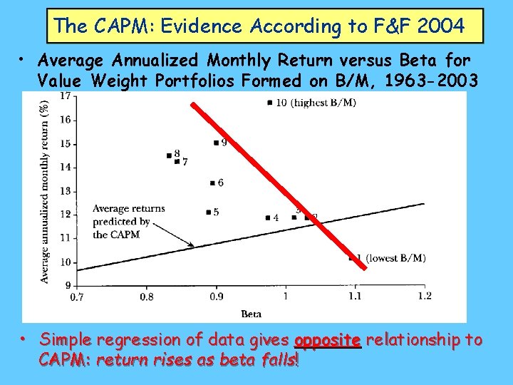
The CAPM: Evidence According to F&F 2004 • “Average returns on the B/M portfolios increase almost monotonically, from 10. 1 percent per year for the lowest B/M group to an impressive 16. 7 percent for the highest. • But the positive relation between beta and average return predicted by the CAPM is notably absent… the portfolio with the lowest book-to-market ratio has the highest beta but the lowest average return. • The estimated beta for the portfolio with the highest book-to marketratio and the highest average return is only 0. 98. With an average annualized value of the riskfree interest rate, Rf, of 5. 8 percent and an average annualized market premium, Rm - Rf, of 11. 3 percent, the Sharpe-Lintner CAPM predicts an average return of 11. 8 percent for the lowest B/M portfolio and 11. 2 percent for the highest, far from the observed values, 10. 1 and 16. 7 percent. ”

The CAPM: Evidence According to F&F 2004 • Average Annualized Monthly Return versus Beta for Value Weight Portfolios Formed on B/M, 1963 -2003 • Simple regression of data gives opposite relationship to CAPM: return rises as beta falls!

“Beta is dead, long live…”? • CAPM clearly a failure – As predictor of stock market behaviour – As guide to formation of return-maximising, riskminimising portfolio • Early “success” possibly due to unusual “financial tranquility” nature of post-WWII to 1966 stock market • New model of finance needed – To explain behaviour of asset markets in general – To guide portfolio selection • Next week: the developing Really New Finance: – The Inefficient Market Hypothesis – The Fractal Market Hypothesis – Chaos, heterogeneity and “minority games”