Event Studies in Financial Economics A Review https

Event Studies in Financial Economics: A Review https: //www. bauer. uh. edu/rsusmel/phd/lecture%206. pdf

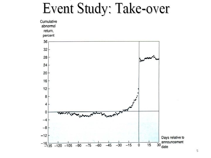
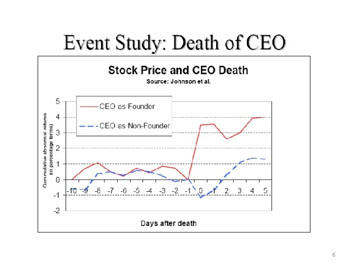
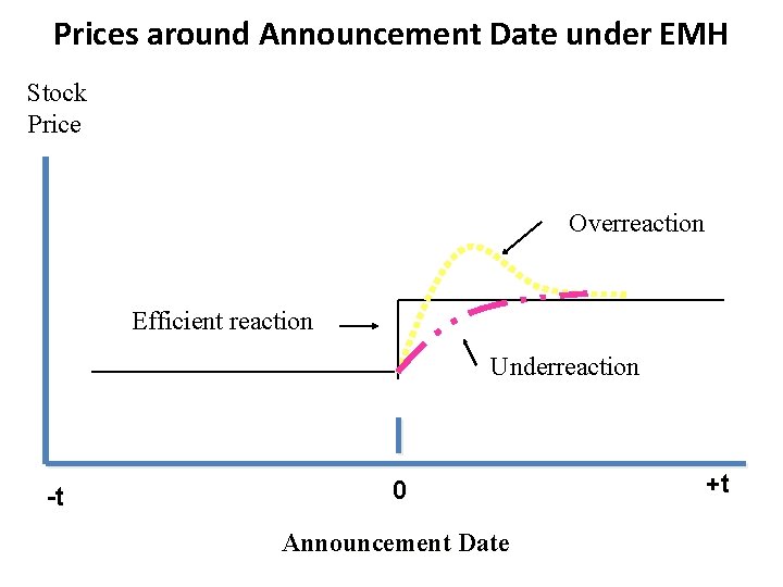
Event Study Analysis • Definition: An event study attempts to measure the valuation effects of an event, such as a merger or earnings announcement, by examining the response of the stock price around the announcement of the event. • One underlying assumption is that the market processes information about the event in an efficient and unbiased manner. • Thus, we should be able to see the effect of the event on prices.

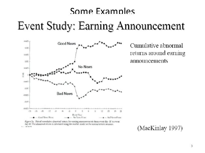
Some Examples 3

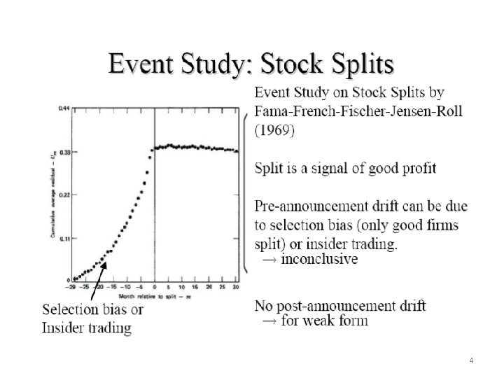
4

5

6

Prices around Announcement Date under EMH Stock Price Overreaction Efficient reaction Underreaction -t 0 Announcement Date +t

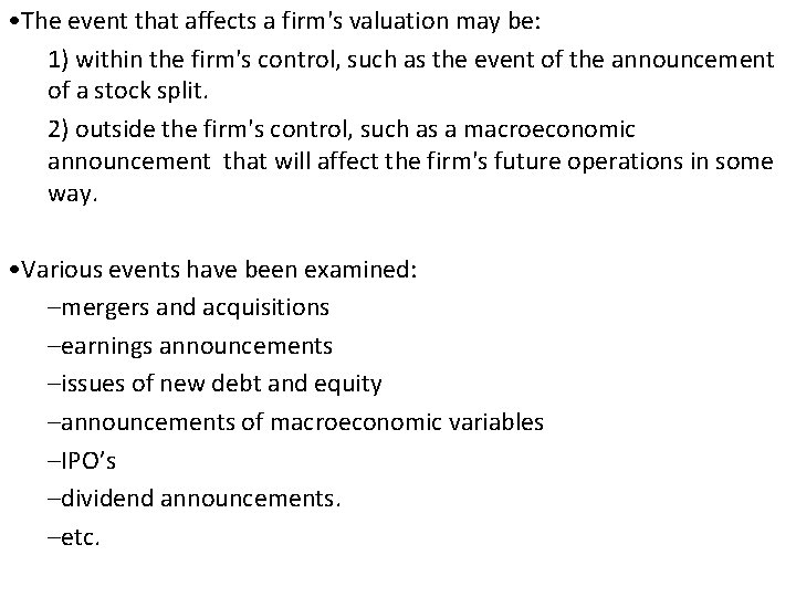
• The event that affects a firm's valuation may be: 1) within the firm's control, such as the event of the announcement of a stock split. 2) outside the firm's control, such as a macroeconomic announcement that will affect the firm's future operations in some way. • Various events have been examined: –mergers and acquisitions –earnings announcements –issues of new debt and equity –announcements of macroeconomic variables –IPO’s –dividend announcements. –etc.

• Technique mainly used in corporate. • Simple on the surface, but there a lot of issues. • Long history in finance: – First paper that applies event-studies, as we know them today: Fama, Fisher, Jensen, and Roll (1969) for stock splits. – Today, we find thousands of papers using event-study methods.

Event Study Design • The steps for an event study are as follows: – Event Definition – Selection Criteria – Normal and Abnormal Return Measurement – Estimation Procedure – Testing Procedure – Empirical Results – Interpretation

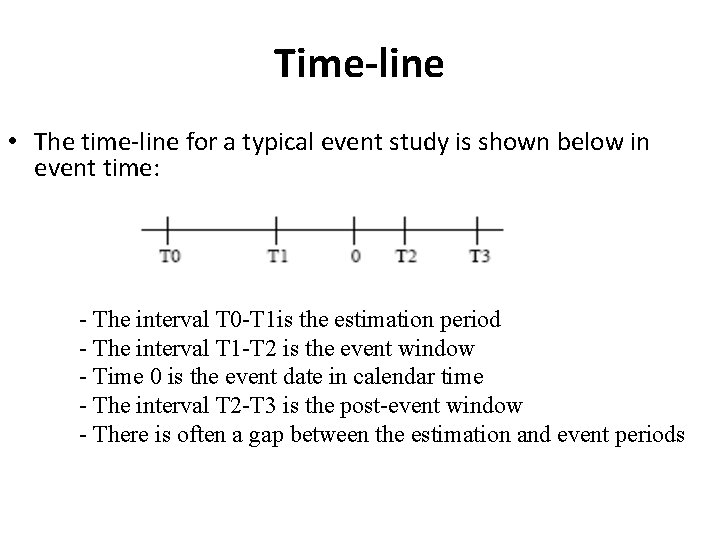
Time-line • The time-line for a typical event study is shown below in event time: - The interval T 0 -T 1 is the estimation period - The interval T 1 -T 2 is the event window - Time 0 is the event date in calendar time - The interval T 2 -T 3 is the post-event window - There is often a gap between the estimation and event periods

• Issues with the Time-line: - Defintion of an event: We have to define what an event is. It must be unexpected. Also, we must know the exact date of the event. Dating is always a problem (WSJ is not a good source -leakage). - Frequency of the event study: We have to decide how fast the information is incorporated into prices. We cannot look at yearly returns. We can’t look at 10 -seconds returns. People usually look at daily, weekly or monthly returns. - Sample Selection: We have to decide what is the universe of companies in the sample. - Horizon of the event study: If markets are efficient, we should consider short horizons –i. e. , a few days. However, people have looked at long-horizons. Event studies can be categorized by horizon: - Short horizon (from 1 -month before to 1 -month after the event) - Long horizon (up to 5 years after the event).

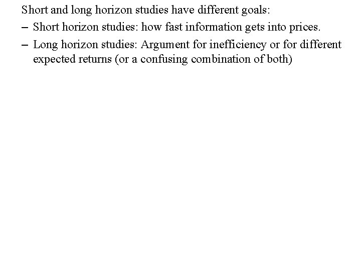
Short and long horizon studies have different goals: – Short horizon studies: how fast information gets into prices. – Long horizon studies: Argument for inefficiency or for different expected returns (or a confusing combination of both)

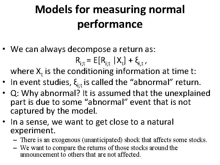
Models for measuring normal performance • We can always decompose a return as: Ri; t = E[Ri; t |Xt] + ξi, t , where Xt is the conditioning information at time t: • In event studies, ξi; t is called the “abnormal” return. • Q: Why abnormal? It is assumed that the unexplained part is due to some “abnormal” event that is not captured by the model. • In a sense, we want to get close to a natural experiment. – There is an exogenous (unanticipated) shock that affects some stocks. – We want to compare the returns of those stocks around the announcement to others that are not affected.

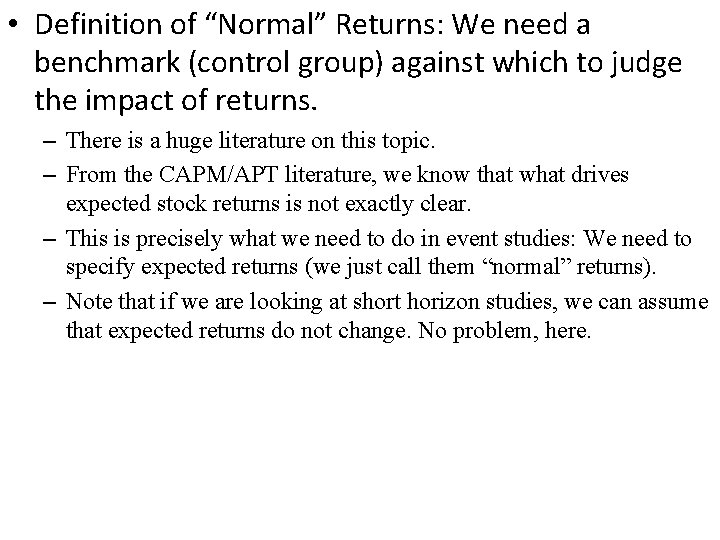
• Definition of “Normal” Returns: We need a benchmark (control group) against which to judge the impact of returns. – There is a huge literature on this topic. – From the CAPM/APT literature, we know that what drives expected stock returns is not exactly clear. – This is precisely what we need to do in event studies: We need to specify expected returns (we just call them “normal” returns). – Note that if we are looking at short horizon studies, we can assume that expected returns do not change. No problem, here.

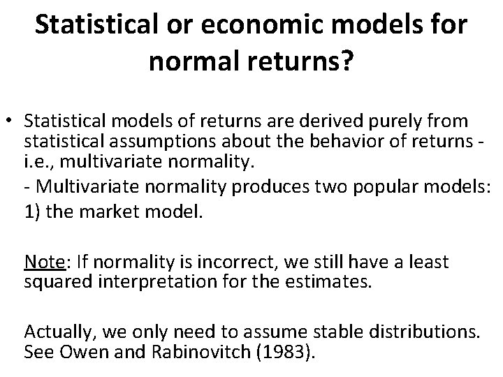
Statistical or economic models for normal returns? • Statistical models of returns are derived purely from statistical assumptions about the behavior of returns i. e. , multivariate normality. - Multivariate normality produces two popular models: 1) the market model. Note: If normality is incorrect, we still have a least squared interpretation for the estimates. Actually, we only need to assume stable distributions. See Owen and Rabinovitch (1983).

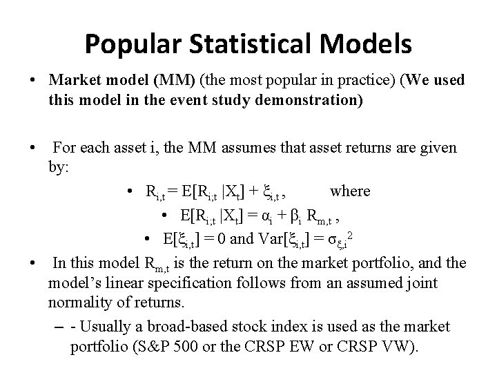
Popular Statistical Models • Market model (MM) (the most popular in practice) (We used this model in the event study demonstration) • For each asset i, the MM assumes that asset returns are given by: • Ri, t = E[Ri; t |Xt] + ξi, t , where • E[Ri; t |Xt] = αi + βi Rm, t , • E[ξi, t] = 0 and Var[ξi, t] = σξ, i 2 • In this model Rm, t is the return on the market portfolio, and the model’s linear specification follows from an assumed joint normality of returns. – - Usually a broad-based stock index is used as the market portfolio (S&P 500 or the CRSP EW or CRSP VW).

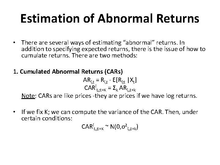
Estimation of Abnormal Returns • There are several ways of estimating “abnormal” returns. In addition to specifying expected returns, there is the issue of how to cumulate returns. There are two methods: 1. Cumulated Abnormal Returns (CARs) ARi, t = Ri, t - E[Ri; t |Xt] CARit, ; t+K = Σk ARi, , t+k Note: CARs are like prices -they are prices if we have log returns. • If we fix K; we can compute the variance of the CAR. Then, under certain conditions: CARit, ; t+K ~ N(0, σ2 i, , t+k)

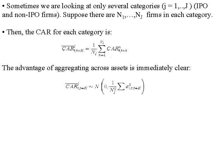
• Sometimes we are looking at only several categories (j = 1, . . , J ) (IPO and non-IPO firms). Suppose there are N 1, …, NJ firms in each category. • Then, the CAR for each category is: The advantage of aggregating across assets is immediately clear:

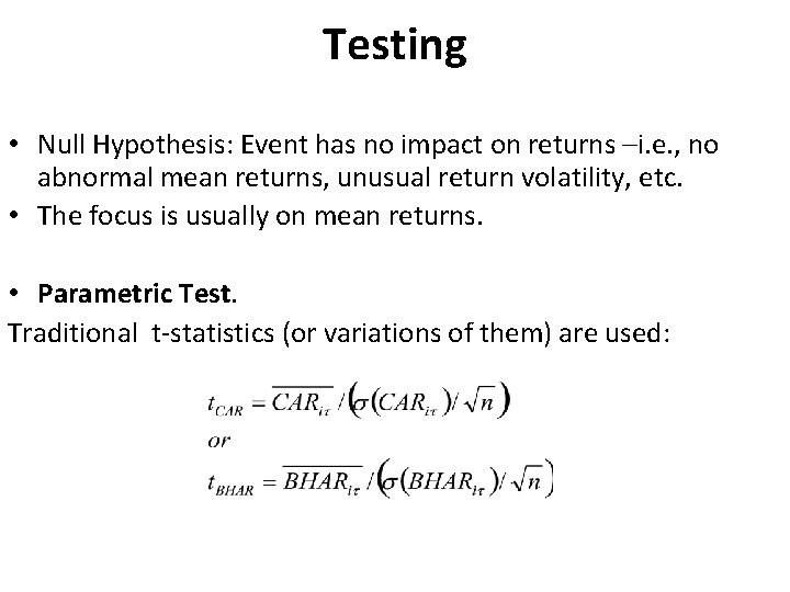
Testing • Null Hypothesis: Event has no impact on returns –i. e. , no abnormal mean returns, unusual return volatility, etc. • The focus is usually on mean returns. • Parametric Test. Traditional t-statistics (or variations of them) are used:

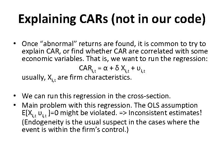
Explaining CARs (not in our code) • Once “abnormal” returns are found, it is common to try to explain CAR, or find whether CAR are correlated with some economic variables. That is, we want to run the regression: CARi, t = α + δ Xi, t + υi, t usually, Xi, t are firm characteristics. • We can run this regression in the cross-section. • Main problem with this regression. The OLS assumption E[Xi, t υi, t ]=0 might be violated. => Inconsistent estimates! (Endogeneity is the usual suspect in the cases where the event is within the firm’s control. )