Linear Program Set Cover Set Cover Given a

Linear Program Set Cover

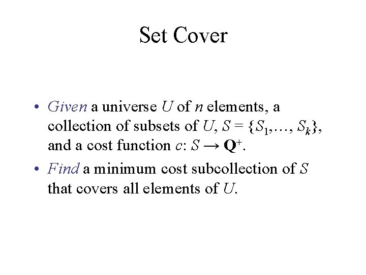
Set Cover • Given a universe U of n elements, a collection of subsets of U, S = {S 1, …, Sk}, and a cost function c: S → Q+. • Find a minimum cost subcollection of S that covers all elements of U.

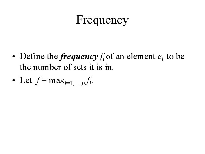
Frequency • Define the frequency fi of an element ei to be the number of sets it is in. • Let f = maxi=1, …, n fi.

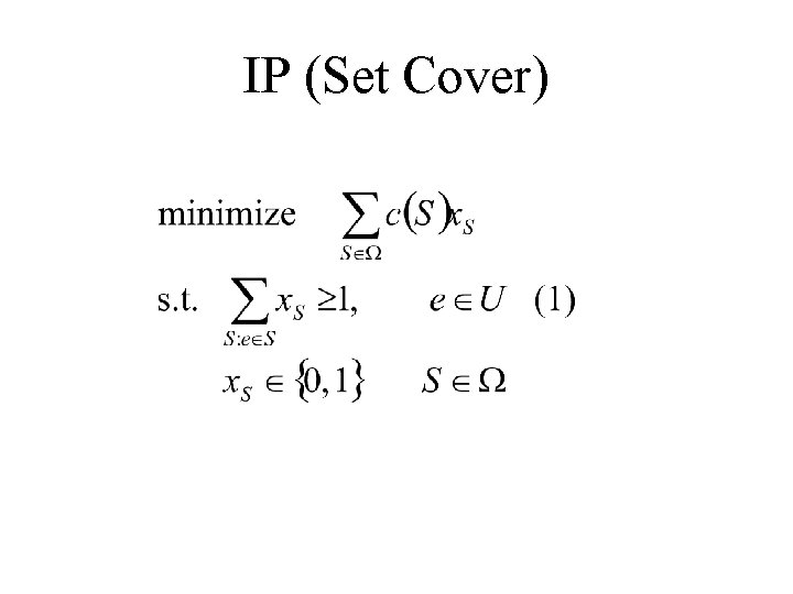
IP (Set Cover)

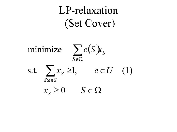
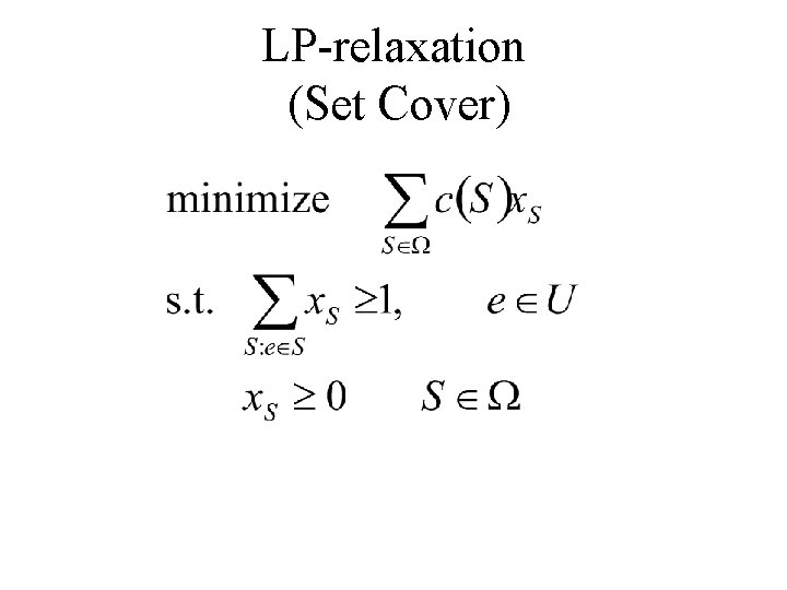
LP-relaxation (Set Cover)

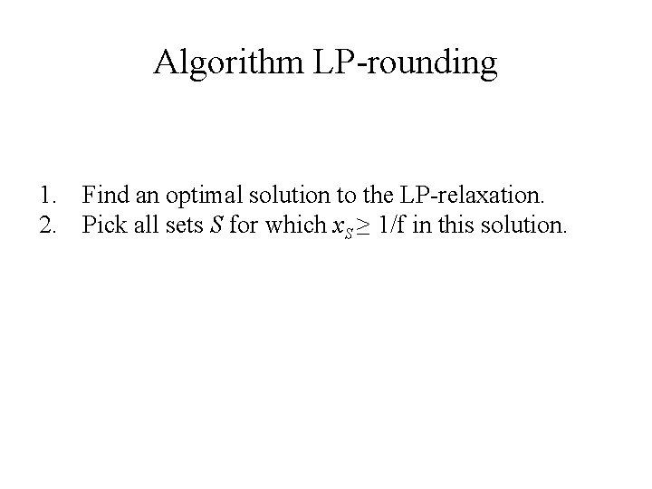
Algorithm LP-rounding 1. Find an optimal solution to the LP-relaxation. 2. Pick all sets S for which x. S ≥ 1/f in this solution.

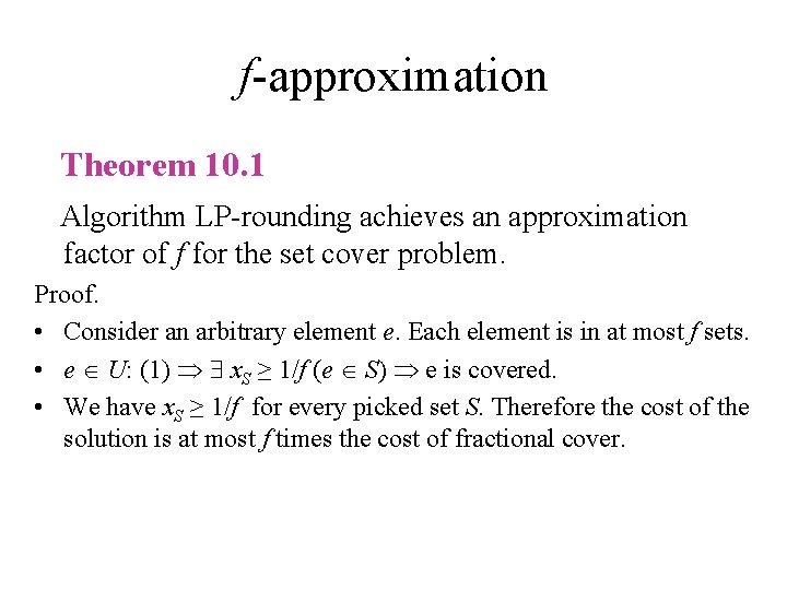
f-approximation Theorem 10. 1 Algorithm LP-rounding achieves an approximation factor of f for the set cover problem. Proof. • Consider an arbitrary element e. Each element is in at most f sets. • e U: (1) x. S ≥ 1/f (e S) e is covered. • We have x. S ≥ 1/f for every picked set S. Therefore the cost of the solution is at most f times the cost of fractional cover.

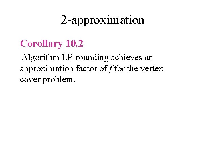
2 -approximation Corollary 10. 2 Algorithm LP-rounding achieves an approximation factor of f for the vertex cover problem.

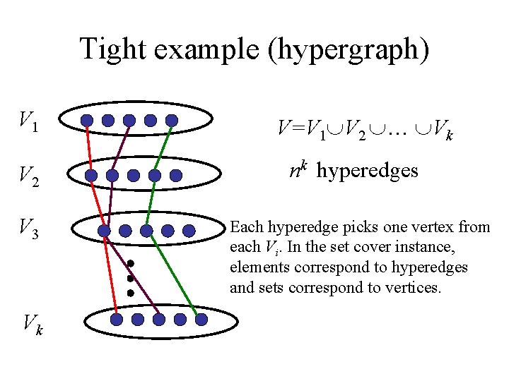
Tight example (hypergraph) V 1 V 2 V 3 Vk V=V 1 V 2 … Vk nk hyperedges Each hyperedge picks one vertex from each Vi. In the set cover instance, elements correspond to hyperedges and sets correspond to vertices.

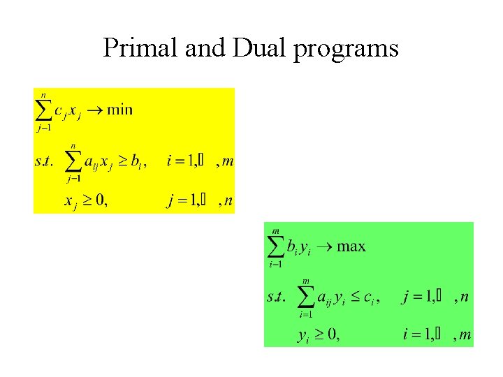
Primal and Dual programs

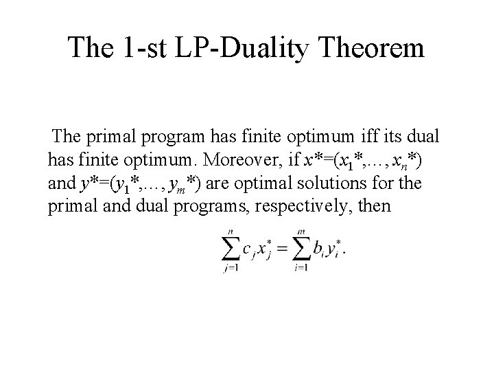
The 1 -st LP-Duality Theorem The primal program has finite optimum iff its dual has finite optimum. Moreover, if x*=(x 1*, …, xn*) and y*=(y 1*, …, ym*) are optimal solutions for the primal and dual programs, respectively, then

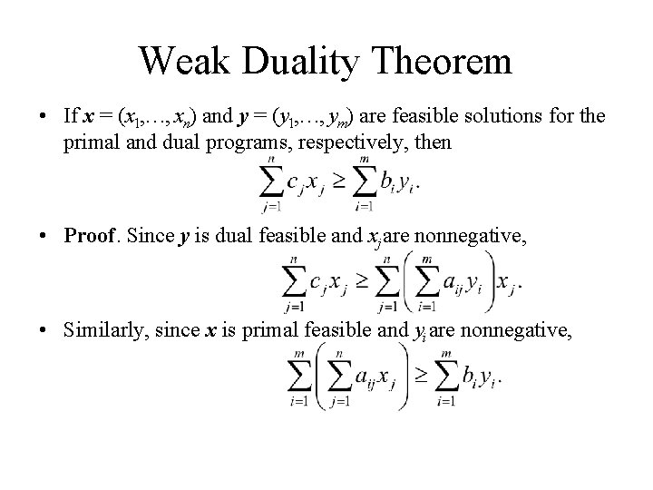
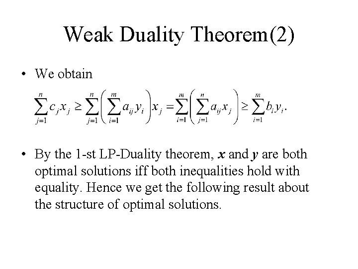
Weak Duality Theorem • If x = (x 1, …, xn) and y = (y 1, …, ym) are feasible solutions for the primal and dual programs, respectively, then • Proof. Since y is dual feasible and xj are nonnegative, • Similarly, since x is primal feasible and yi are nonnegative,

Weak Duality Theorem(2) • We obtain • By the 1 -st LP-Duality theorem, x and y are both optimal solutions iff both inequalities hold with equality. Hence we get the following result about the structure of optimal solutions.

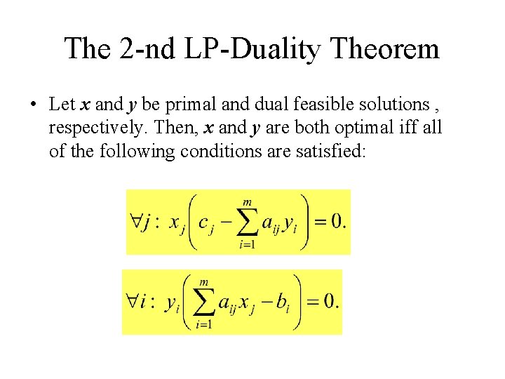
The 2 -nd LP-Duality Theorem • Let x and y be primal and dual feasible solutions , respectively. Then, x and y are both optimal iff all of the following conditions are satisfied:

Primal-Dual Schema • The primal-dual schema is the method of choice for designing approximation algorithms since it yields combinatorial algorithms with good approximation factors and good running times. • We will first present the central ideas behind this schema and then use it to design a simple f factor algorithm for set cover, where f is the frequency of the most frequent element.

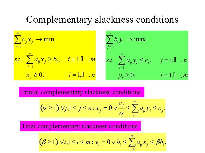
Complementary slackness conditions Primal complementary slackness conditions Dual complementary slackness conditions

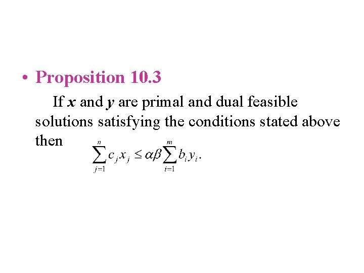
• Proposition 10. 3 If x and y are primal and dual feasible solutions satisfying the conditions stated above then

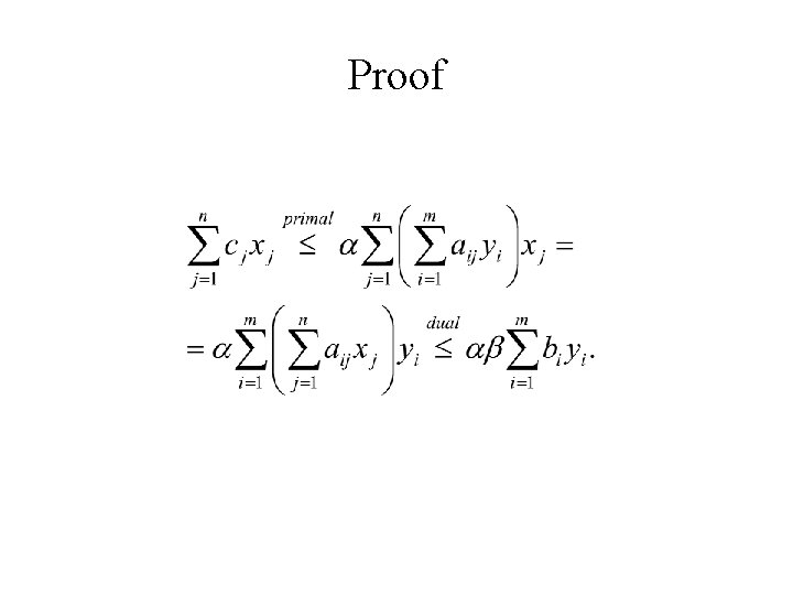
Proof

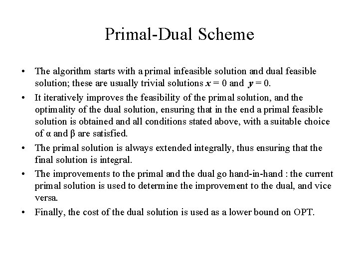
Primal-Dual Scheme • The algorithm starts with a primal infeasible solution and dual feasible solution; these are usually trivial solutions x = 0 and y = 0. • It iteratively improves the feasibility of the primal solution, and the optimality of the dual solution, ensuring that in the end a primal feasible solution is obtained and all conditions stated above, with a suitable choice of α and β are satisfied. • The primal solution is always extended integrally, thus ensuring that the final solution is integral. • The improvements to the primal and the dual go hand-in-hand : the current primal solution is used to determine the improvement to the dual, and vice versa. • Finally, the cost of the dual solution is used as a lower bound on OPT.

LP-relaxation (Set Cover)

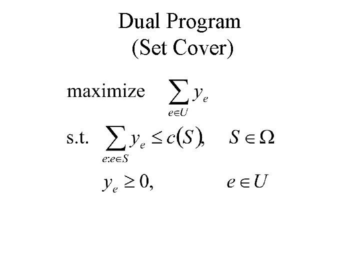
Dual Program (Set Cover)

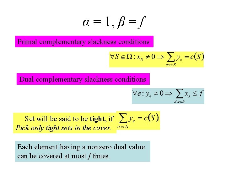
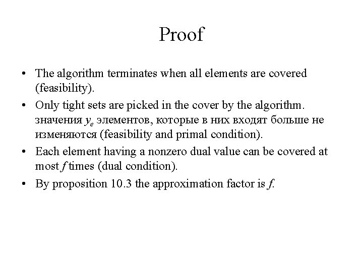
α = 1, β = f Primal complementary slackness conditions Dual complementary slackness conditions Set will be said to be tight, if Pick only tight sets in the cover. Each element having a nonzero dual value can be covered at most f times.

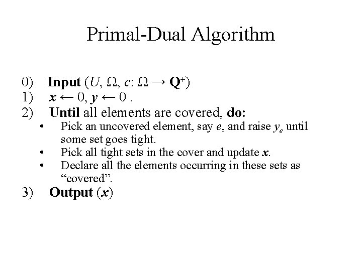
Primal-Dual Algorithm 0) Input (U, Ω, c: Ω → Q+) 1) x ← 0, y ← 0. 2) Until all elements are covered, do: • • • 3) Pick an uncovered element, say e, and raise ye until some set goes tight. Pick all tight sets in the cover and update x. Declare all the elements occurring in these sets as “covered”. Output (x)

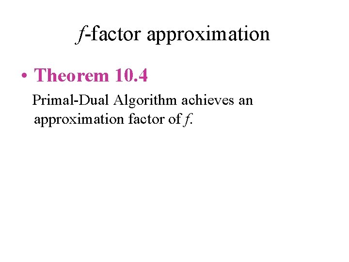
f-factor approximation • Theorem 10. 4 Primal-Dual Algorithm achieves an approximation factor of f.

Proof • The algorithm terminates when all elements are covered (feasibility). • Only tight sets are picked in the cover by the algorithm. значения ye элементов, которые в них входят больше не изменяются (feasibility and primal condition). • Each element having a nonzero dual value can be covered at most f times (dual condition). • By proposition 10. 3 the approximation factor is f.

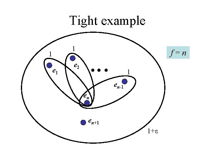
Tight example 1 1 e 1 f=n e 2 1 en-1 en en+1 1+ε

Maximum Satisfiability (MAX-SAT) • Given a conjunctive normal formula f on Boolean variables x 1, …, xn, and nonnegative weights wc, for each clause c of f. • Find a truth assignment to the Boolean variables that maximizes the total weight of satisfied clauses.

Clauses • Each clause is a disjunction of literals; each literal being either a Boolean variable or its negation. Let size(c) denote the size of clause c, i. e. , the number of literals in it. We will assume that the sizes of clauses in f are arbitrary. • A clause is said to be satisfied if one of the unnegated variables is set to true or one of the negated variables is set to false.

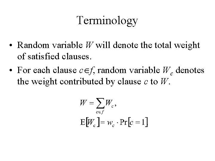
Terminology • Random variable W will denote the total weight of satisfied clauses. • For each clause c f, random variable Wc denotes the weight contributed by clause c to W.

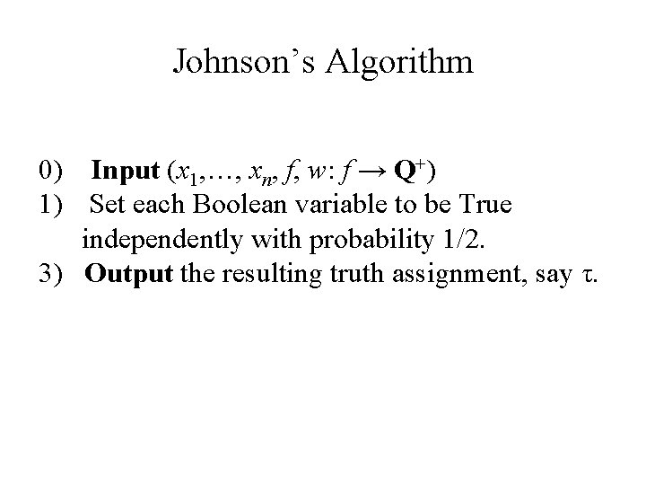
Johnson’s Algorithm 0) Input (x 1, …, xn, f, w: f → Q+) 1) Set each Boolean variable to be True independently with probability 1/2. 3) Output the resulting truth assignment, say τ.

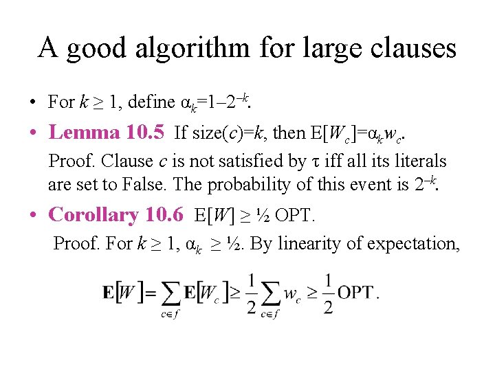
A good algorithm for large clauses • For k ≥ 1, define αk=1– 2–k. • Lemma 10. 5 If size(c)=k, then E[Wc]=αkwc. Proof. Clause c is not satisfied by τ iff all its literals are set to False. The probability of this event is 2–k. • Corollary 10. 6 E[W] ≥ ½ OPT. Proof. For k ≥ 1, αk ≥ ½. By linearity of expectation,

Conditional Expectation • Let a 1, …, ai be a truth assignment to x 1, …, xi. • Lemma 10. 7 E[W| x 1= a 1, …, xi = ai] can be computed in polynomial time.

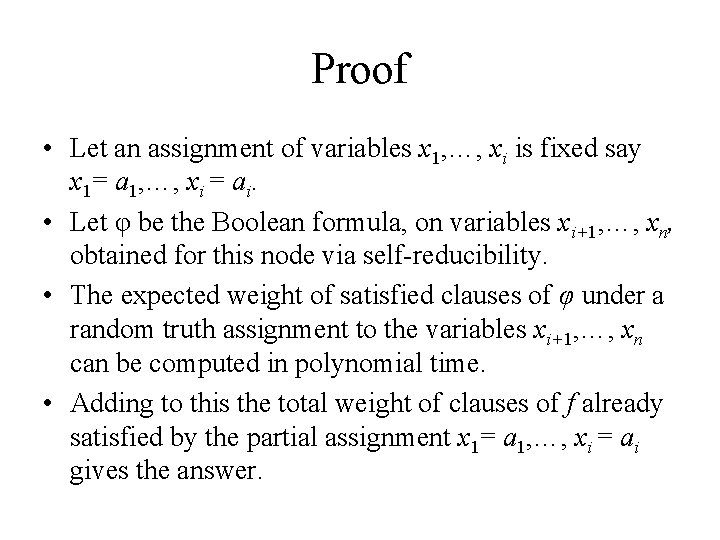
Proof • Let an assignment of variables x 1, …, xi is fixed say x 1= a 1, …, xi = ai. • Let φ be the Boolean formula, on variables xi+1, …, xn, obtained for this node via self-reducibility. • The expected weight of satisfied clauses of φ under a random truth assignment to the variables xi+1, …, xn can be computed in polynomial time. • Adding to this the total weight of clauses of f already satisfied by the partial assignment x 1= a 1, …, xi = ai gives the answer.

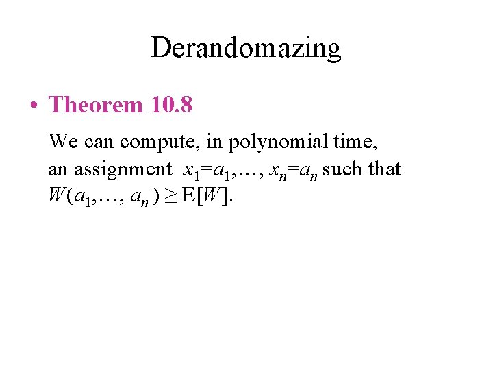
Derandomazing • Theorem 10. 8 We can compute, in polynomial time, an assignment x 1=a 1, …, xn=an such that W(a 1, …, an ) ≥ E[W].

Proof • E[W| x 1=a 1, …, xi=ai] = E[W| x 1=a 1, …, xi=ai, xi+1= True]/2 + + E[W| x 1=a 1, …, xi=ai, xi+1= False]/2 • It follows that either E[W| x 1=a 1, …, xi=ai, xi+1= True] ≥ E[W| x 1=a 1, …, xi=ai], or E[W| x 1=a 1, …, xi=ai, xi+1= False] ≥ E[W| x 1=a 1, …, xi=ai]. • Take an assignment with larger expectation. • The procedure requires n iterations. Lemma 10. 7 implies that each iteration can be done in polynomial time.

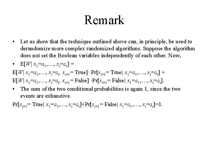
Remark • Let us show that the technique outlined above can, in principle, be used to derandomize more complex randomized algorithms. Suppose the algorithm does not set the Boolean variables independently of each other. Now, • E[W| x 1=a 1, …, xi=ai] = E[W| x 1=a 1, …, xi=ai, xi+1= True] ·Pr[xi+1= True| x 1=a 1, …, xi=ai] + E[W| x 1=a 1, …, xi=ai, xi+1= False] ·Pr[xi+1= False| x 1=a 1, …, xi=ai]. • The sum of the two conditional probabilities is again 1, since the two events are exhaustive. Pr[xi+1= True| x 1=a 1, …, xi=ai]+Pr[xi+1= False| x 1=a 1, …, xi=ai]=1.

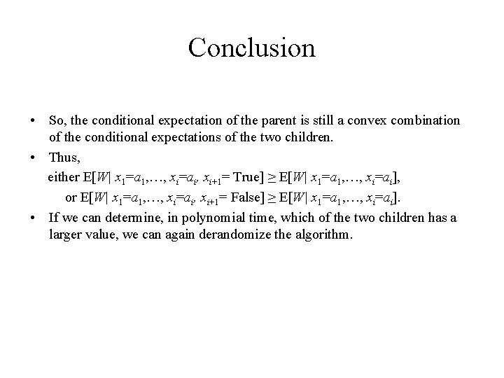
Conclusion • So, the conditional expectation of the parent is still a convex combination of the conditional expectations of the two children. • Thus, either E[W| x 1=a 1, …, xi=ai, xi+1= True] ≥ E[W| x 1=a 1, …, xi=ai], or E[W| x 1=a 1, …, xi=ai, xi+1= False] ≥ E[W| x 1=a 1, …, xi=ai]. • If we can determine, in polynomial time, which of the two children has a larger value, we can again derandomize the algorithm.

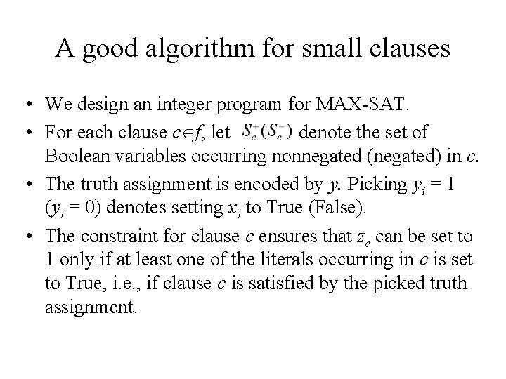
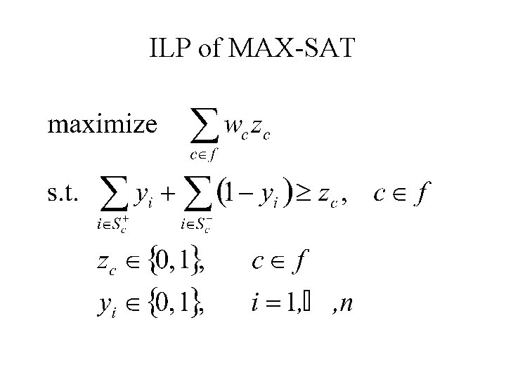
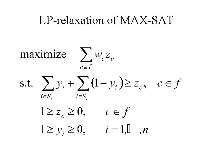
A good algorithm for small clauses • We design an integer program for MAX-SAT. • For each clause c f, let denote the set of Boolean variables occurring nonnegated (negated) in c. • The truth assignment is encoded by y. Picking yi = 1 (yi = 0) denotes setting xi to True (False). • The constraint for clause c ensures that zc can be set to 1 only if at least one of the literals occurring in c is set to True, i. e. , if clause c is satisfied by the picked truth assignment.

ILP of MAX-SAT

LP-relaxation of MAX-SAT

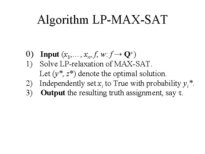
Algorithm LP-MAX-SAT 0) Input (x 1, …, xn, f, w: f → Q+) 1) Solve LP-relaxation of MAX-SAT. Let (y*, z*) denote the optimal solution. 2) Independently set xi to True with probability yi*. 3) Output the resulting truth assignment, say τ.

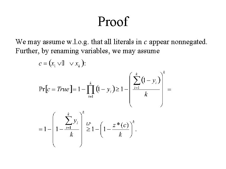
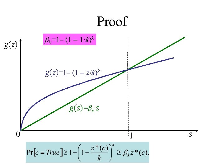
Expected weight of disjunction • For k ≥ 1, define βk=1– (1 – 1/k)k. • Lemma 10. 9 If size(c)=k, then E[Wc] ≥ βkwcz*(c).

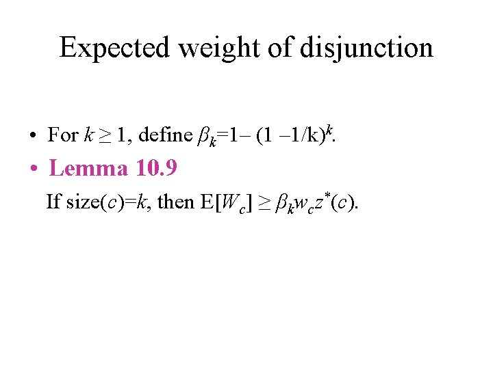
Proof We may assume w. l. o. g. that all literals in c appear nonnegated. Further, by renaming variables, we may assume

Proof g(z) βk=1– (1 – 1/k)k g(z)=1– (1 – z/k)k g(z)=βk·z 0 1 z

1– 1/e • Corollary 10. 10 E[W] ≥ βk. OPT (if all clauses are of size at most k). • Proof. Notice that βk is a decreasing function of k. Thus, if all clauses are of size at most k,

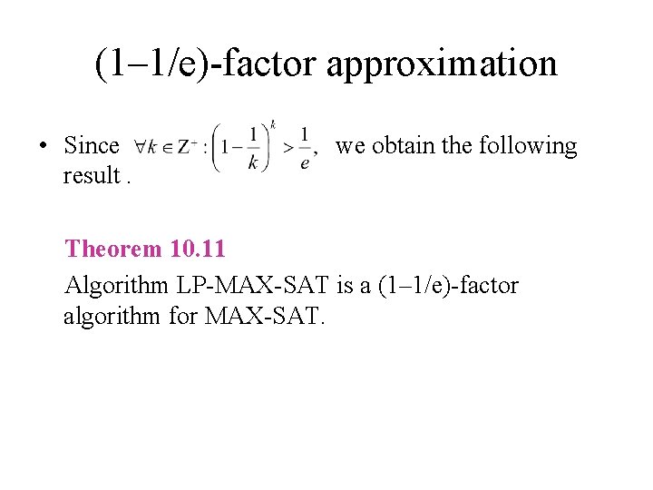
(1– 1/e)-factor approximation • Since result. we obtain the following Theorem 10. 11 Algorithm LP-MAX-SAT is a (1– 1/e)-factor algorithm for MAX-SAT.

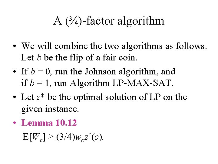
A (¾)-factor algorithm • We will combine the two algorithms as follows. Let b be the flip of a fair coin. • If b = 0, run the Johnson algorithm, and if b = 1, run Algorithm LP-MAX-SAT. • Let z* be the optimal solution of LP on the given instance. • Lemma 10. 12 E[Wc] ≥ (3/4)wcz*(c).

E[Wc] ≥ (3/4)wcz*(c) • • Let size(c)=k. Л 8. 5 E[Wc|b=0] = αkwc ≥ αkwc z*(c) Л 8. 9 E[Wc|b=1] ≥ βkwc z*(c) E[Wc] = (1/2)(E[Wc|b=0]+ E[Wc|b=1]) ≥ ≥ (1/2)wc z*(c)(αk+βk) • α 1+ β 1 = α 2+ β 2 = 3/2 • k ≥ 3, αk+ βk ≥ 7/8 + (1– 1/e) > 3/2 • E[Wc] ≥ (3/4)wcz*(c)

E[W] By linearity of expectation, Finally, consider the following deterministic algorithm.

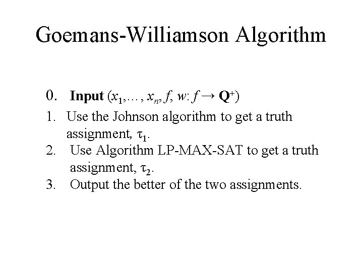
Goemans-Williamson Algorithm 0. Input (x 1, …, xn, f, w: f → Q+) 1. Use the Johnson algorithm to get a truth assignment, τ1. 2. Use Algorithm LP-MAX-SAT to get a truth assignment, τ2. 3. Output the better of the two assignments.

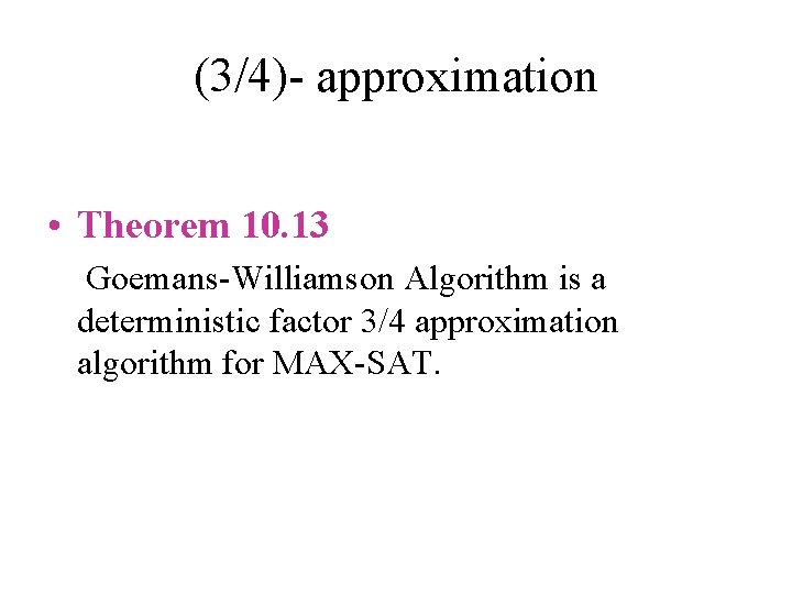
(3/4)- approximation • Theorem 10. 13 Goemans-Williamson Algorithm is a deterministic factor 3/4 approximation algorithm for MAX-SAT.

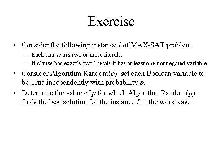
Exercise • Consider the following instance I of MAX-SAT problem. – Each clause has two or more literals. – If clause has exactly two literals it has at least one nonnegated variable. • Consider Algorithm Random(p): set each Boolean variable to be True independently with probability p. • Determine the value of p for which Algorithm Random(p) finds the best solution for the instance I in the worst case.