Limits and Their Properties A Preview of Calculus

Limits and Their Properties

A Preview of Calculus

What Is Calculus?

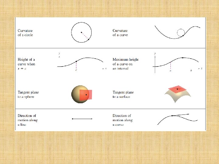
Calculus is the mathematics of change. Calculus is the mathematics of velocities, accelerations, tangent lines, slopes, areas, volumes, arc lengths, centroids, curvatures, and a variety of other concepts that have enabled scientists, engineers, and economists to model real-life situations. Although precalculus mathematics also deals with velocities, accelerations, tangent lines, slopes, and so on, there is a fundamental difference between precalculus mathematics and calculus. Precalculus mathematics is more static, whereas calculus is more dynamic.

So, one way to answer the question “What is calculus? ” is to say that calculus is a “limit machine” that involves three stages. 1. The first stage is precalculus mathematics, such as the slope of a line or the area of a rectangle. 2. The second stage is the limit process 3. The third stage is a new calculus formulation, such as a derivative or integral.

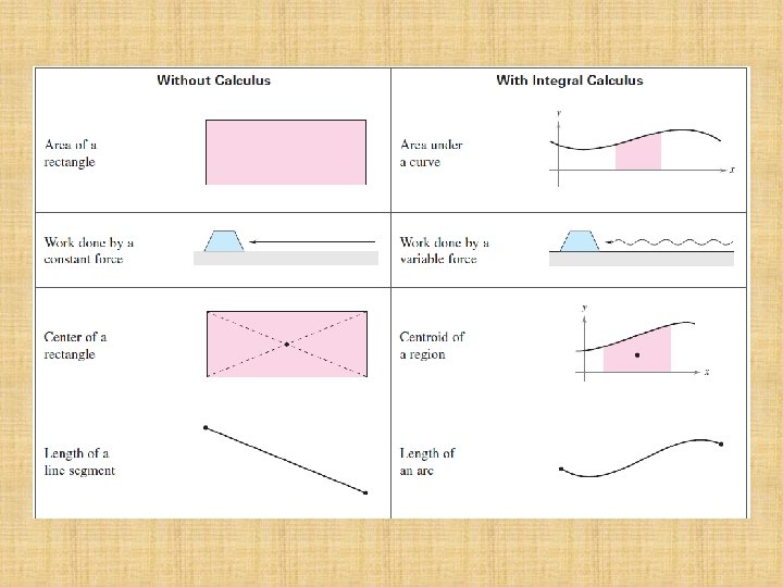
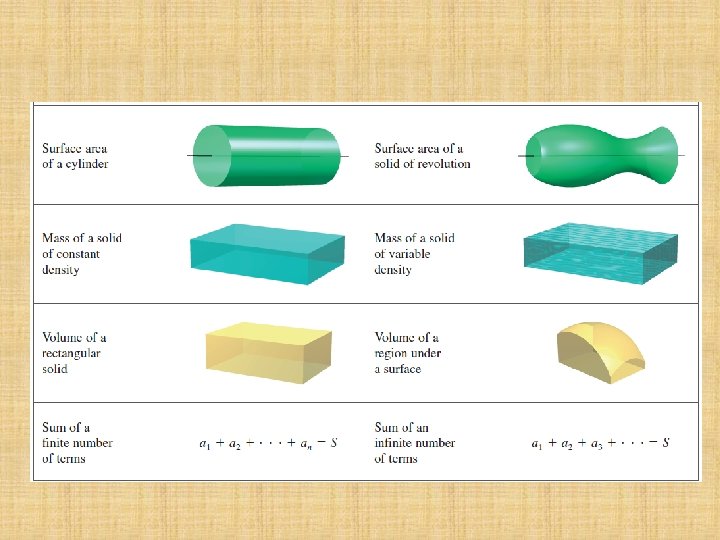
Here are some familiar precalculus concepts coupled their calculus counterparts:

Finding Limits Graphically and Numerically

An Introduction to Limits

An Introduction to Limits To sketch the graph of the function for values other than x = 1, you can use standard curve-sketching techniques. At x = 1, however, it is not clear what to expect.

To get an idea of the behavior of the graph of f near x = 1, you can use two sets of x-values–one set that approaches 1 from the left and one set that approaches 1 from the right, as shown in the table.

Although x can not equal 1, you can move arbitrarily close to 1 from both sides, and as a result f(x) moves arbitrarily close to 3. Using limit notation, you can write This is read as “the limit of f(x) as x approaches 1 is 3. ”

This discussion leads to an informal definition of limit. If f(x) becomes arbitrarily close to a single number L as x approaches c from either side, the limit of f(x), as x approaches c, is L. This limit is written as

Example 1 – Estimating a Limit Numerically Evaluate the function at several points near x = 0 and use the results to estimate the limit

Example 1 – Solution The table lists the values of f(x) for several x-values near 0.

Example 1 – Solution From the results shown in the table, you can estimate the limit to be 2. This limit is reinforced by the graph of f cont’d

Three pronged approach to problem solving (finding limits) 1. Numerical approach - Construct a table of values 2. Graphical approach - Draw a graph by hand or using technology 3. Analytic approach - Use algebra or calculus

Limits That Fail to Exist Common Types of Behavior Associated with Nonexistence of a Limit: 1. f(x) approaches a different number from the right side of c that is approaches from the left side. 2. f(x) increases or decreases without bound as x approaches c. 3. f(x) oscillates between two fixed values as x approaches c.

Example 3 – Different Right and Left Behavior Show that the limit does not exist. Solution: Consider the graph of the function In Figure and from the definition of absolute value, you can see that

Example 4 – Increases without bound

Example 5 – Oscillates

A Formal Definition of Limit

A Formal Definition of Limit Let’s take another look at the informal definition of limit. If f(x) becomes arbitrarily close to a single number L as x approaches c from either side, then the limit of f(x) as x approaches c is L, is written as At first glance, this definition looks fairly technical. Even so, it is informal because exact meanings have not yet been given to the two phrases “f(x) becomes arbitrarily close to L” and “x approaches c. ”

A Formal Definition of Limit The first person to assign mathematically rigorous meanings to these two phrases was Augustin-Louis Cauchy. His definition of limit is the standard used today. In Figure 1. 12, let (the lower case Greek letter epsilon) represent (small) positive number. a Then the phrase “f(x) becomes arbitrarily close to L” means that f(x) lies in the interval (L – , L + ). Figure 1. 12

A Formal Definition of Limit Using absolute value, you can write this as Similarly, the phrase “x approaches c” means that there exists a positive number such that x lies in either the interval or the interval This fact can be concisely expressed by the double inequality

A Formal Definition of Limit

Example 6 – - PROOF Use the formal definition of a limit to prove Solution: You must show that for each ε > 0 there exists a δ > 0 such that if then Here we need to work with the and relate it to to see the relationship between ε and δ.

This is how the proof should be written formally: Given ε let δ=ε/3 then Q. E. D.

Evaluating Limits Analytically

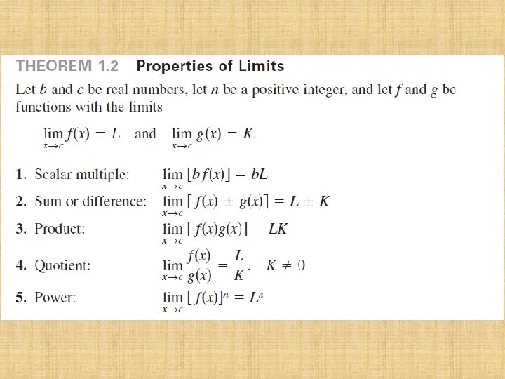
Properties of Limits

The limit of f (x) as x approaches c does not depend on the value of f at x = c. It may happen, however, that the limit is precisely f (c). In such cases, the limit can be evaluated by direct substitution. That is, Such well-behaved functions are continuous at c.

Let b and c be real numbers

Example 1 – Evaluating Basic Limits

Example 2 – The Limit of a Polynomial Solution:

The limit (as x → 2 ) of the polynomial function p(x) = 4 x 2 + 3 is simply the value of p at x = 2. This direct substitution property is valid for all polynomial and rational functions with nonzero denominators.

Example 3 – The Limit of a Rational Function Find the limit: Solution: Because the denominator is not 0 when x = 1, you can apply Theorem 1. 3 to obtain

Limits of Polynomials and Rational Functions: If p(x) and q(x) are polynomials and c is a real number, then and , as long as

The Limit of a Function Containing a Radical: Let n be a positive integer. The following limit is valid for all c if n is odd, and is valid for c > 0 if n is even.

Limits of Trigonometric Functions: Let c be a real number in the domain of the given trigonometric function.

Example 4 – Limits of Trigonometric Functions

Its not always this easy! Most limits you come across will not be done with direct substitution.

Functions That Agree at All But One Point: Let c be a real number and let f(x) = g(x) for all x≠c in an open interval containing c. If the limit of g(x) as x approaches c exists, then the limit of f(x) also exists and

Example 6 – Finding the Limit of a Function Find the limit: Solution: Let f (x) = (x 3 – 1) /(x – 1) By factoring and dividing out like factors, you can rewrite f as

Example 6 – Solution So, for all x-values other than x = 1, the functions f and g agree, as shown in Figure 1. 17 f and g agree at all but one point Figure 1. 17 cont’d

Example 6 – Solution Because exists, you can apply Theorem 1. 7 to conclude that f and g have the same limit at x = 1. cont’d

Ex: Find the limit analytically, it is exists

A Strategy for Finding Limits 1. Learn to recognize which limits can be evaluated by direct substitution 2. If the limit of f(x) as x approaches c cannot be evaluated by direct substitution, try to find a function g that agrees with f for all x other than x = c. 3. Apply the previous theorem to conclude analytically that 4. Use a graph or table to reinforce your conclusion

Example 7 – Dividing Out Technique Find the limit: Solution: Although you are taking the limit of a rational function, you cannot apply Theorem 1. 3 because the limit of the denominator is 0.

Example 7 – Solution cont’d Because the limit of the numerator is also 0, the numerator and denominator have a common factor of (x + 3). So, for all x ≠ – 3, you can divide out this factor to obtain Using Theorem 1. 7, it follows that

Example 7 – Solution cont’d This result is shown graphically in Figure 1. 18. Note that the graph of the function f coincides with the graph of the function g(x) = x – 2, except that the graph of f has a gap at the point (– 3, – 5). Figure 1. 18

Rationalizing Technique Another way to find a limit analytically is the rationalizing technique, which involves rationalizing the numerator of a fractional expression. Recall that rationalizing the numerator means multiplying the numerator and denominator by the conjugate of the numerator. For instance, to rationalize the numerator of multiply the numerator and denominator by the conjugate of which is

Example 8 – Rationalizing Technique Find the limit: Solution: By direct substitution, you obtain the indeterminate form 0/0.

Example 8 – Solution In this case, you can rewrite the fraction by rationalizing the numerator. cont’d

Example 8 – Solution Now, using Theorem 1. 7, you can evaluate the limit as shown. cont’d

Example 8 – Solution A table or a graph can reinforce your conclusion that the limit is 1/2. (See Figure 1. 20. ) Figure 1. 20 cont’d

Example 8 – Solution cont’d

These simple technics from algebra (factoring, canceling, rationalizing) don’t always work either!

The Squeeze Theorem The next theorem concerns the limit of a function that is squeezed between two other functions, each of which has the same limit at a given x-value, as shown in Figure 1. 21

The Squeeze Theorem For h(x)≤f(x)≤g(x) for all x in an open interval containing c, except possibly at c itself, and if then exists and is also equal to L. The Squeeze Theorem is also called the Sandwich Theorem or the Pinching Theorem.

Example 9 – A Limit Involving a Trigonometric Function Find the limit: Solution: Direct substitution yields the indeterminate form 0/0. To solve this problem, you can write tan x as (sin x)/(cos x) and obtain

Example 9 – Solution Now, because you can obtain cont’d

Example 9 – Solution (See Figure 1. 23. ) Figure 1. 23 cont’d

Continuity and One-Sided Limits

Continuity at a Point and on an Open Interval

Continuity at a Point and on an Open Interval In mathematics, the term continuous has much the same meaning as it has in everyday usage. Informally, to say that a function f is continuous at x = c means that there is no interruption in the graph of f at c. That is, its graph is unbroken at c and there are no holes, jumps, or gaps.

Continuity at a Point and on an Open Interval Figure 1. 25 identifies three values of x at which the graph of f is not continuous. At all other points in the interval (a, b), the graph of f is uninterrupted and continuous. Figure 1. 25

Continuity at a Point and on an Open Interval

Ex: Show that is continuous at x = 2

Continuity at a Point and on an Open Interval Consider an open interval I that contains a real number c. If a function f is defined on I (except possibly at c), and f is not continuous at c, then f is said to have a discontinuity at c. Discontinuities fall into two categories: removable and nonremovable. A discontinuity at c is called removable if f can be made continuous by appropriately defining (or redefining f(c)).

Continuity at a Point and on an Open Interval For instance, the functions shown in Figures 1. 26(a) and (c) have removable discontinuities at c and the function shown in Figure 1. 26(b) has a nonremovable discontinuity at c. Figure 1. 26

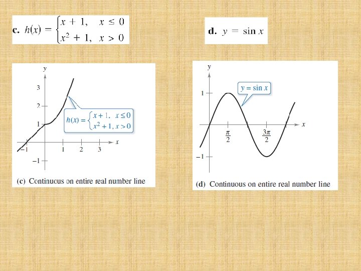
Example 1 – Continuity of a Function Discuss the continuity of each function.

One-Sided Limits To understand continuity on a closed interval, you first need to look at a different type of limit called a one-sided limit. For example, the limit from the right (or right-hand limit) means that x approaches c from values greater than c This limit is denoted as

One-Sided Limits Similarly, the limit from the left (or left-hand limit) means that x approaches c from values less than c. This limit is denoted as

Example 2 – A One-Sided Limit Find the limit of f(x) = right. as x approaches – 2 from the Solution: As shown in Figure 1. 29, the limit as x approaches – 2 from the right is Figure 1. 29

One-Sided Limits One-sided limits can be used to investigate the behavior of step functions. One common type of step function is the greatest integer function , defined by For instance, and

When the limit from the left is not equal to the limit from the right, the (two-sided) limit does not exist. The next theorem makes this more explicit.

One-Sided Limits and Continuity on a Closed Interval Figure 1. 31

Example 4 – Continuity on a Closed Interval Discuss the continuity of f(x) = Solution: The domain of f is the closed interval [– 1, 1]. At all points in the open interval (– 1, 1), the continuity of f follows from Theorems 1. 4 and 1. 5.

Example 4 – Solution cont’d Moreover, because and you can conclude that f is continuous on the closed interval [– 1, 1], as shown in Figure 1. 32

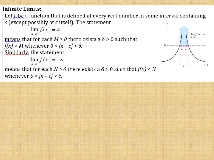
Infinite Limits

Consider the function f(x)= 3/(x – 2). From Figure 1. 39 and the table, you can see that f(x) decreases without bound as x approaches 2 from the left, and f(x) increases without bound as x approaches 2 from the right.

The best way to find a vertical asymptote for a simple rational function is to find all the values for which the denominators are equal to zero but the numerators are NOT.