Introduction to Seasonal Adjustment and JDemetra ESTP course

Introduction to Seasonal Adjustment and JDemetra+ ESTP course EUROSTAT 26 – 28 Janaury 2016 Dario Buono (Eurostat, Methodology in Official Statistics Veronique Elter (STATEC, Quarterly National Accounts) © 2015 by EUROSTAT. All rights reserved. Open to the public

Plan – Day 1 • Morning: • • • Brief overview of Time Series Analysis Seasonality and its determinants Decomposition models Exploration tools Why Seasonal Adjustment? Step by step procedures for SA • Afternoon: • Using JDemetra+ • Getting familiar • First results • Question time for face-to-face discussion with the trainers

Plan – Day 2 • Morning: • Identification of types of outliers: • Calendar Effect and its determinants • • X-13 ARIMA vs. Tramo/Seats How to use the ESS guidelines on SA • Afternoon: • Using JDemetra+ • Calendar Adjustment • Outliers • Question time for face-to-face discussion with the trainers

Plan – day 3 • Morning: • Using JDemetra+ • • Full exercise with ESTAT series Full exercise with MS series • Afternoon: • Using JDemetra+ • Show and tell exercise by participants • Conclusions and evaluation of the course

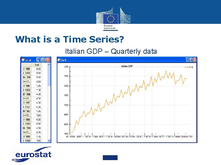
What is a Time Series? n A Time Series is a sequence of measures of a given phenomenon taken at regular time intervals such as hourly, daily, weekly, monthly, quarterly, annually, or every so many years – Stock series are measures of activity at a point in time and can be thought of as stocktakes (e. g. the Monthly Labour Force Survey takes stock of whether a person was employed in the reference week) – Flow series are series which are a measure of activity to a date (e. g. Retail, Current Account Deficit, Balance of Payments)

What is a Time Series? Italian GDP – Quarterly data

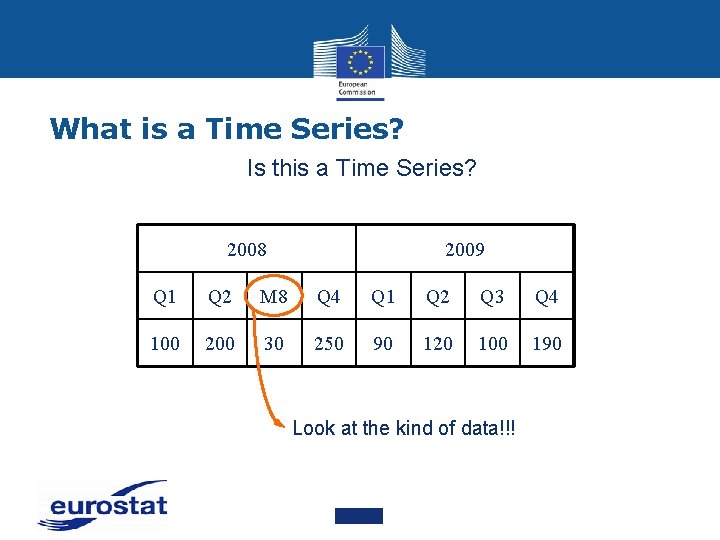
What is a Time Series? Is this a Time Series? 2008 2009 Q 1 Q 2 M 8 Q 4 Q 1 Q 2 Q 3 Q 4 100 200 30 250 90 120 100 190 Look at the kind of data!!!

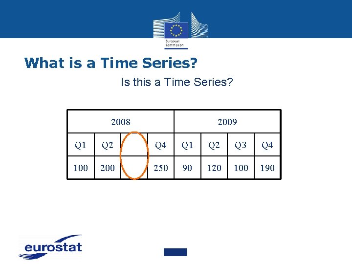
What is a Time Series? Is this a Time Series? 2008 2009 Q 1 Q 2 Q 4 Q 1 Q 2 Q 3 Q 4 100 250 90 120 100 190

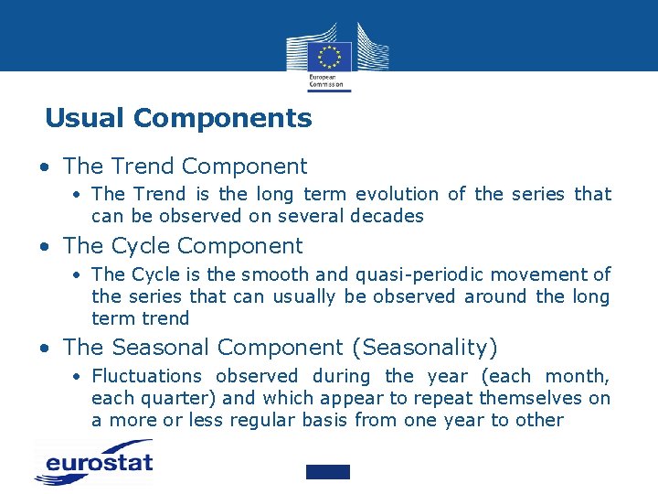
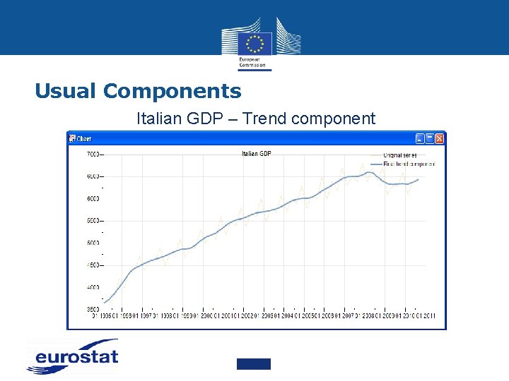
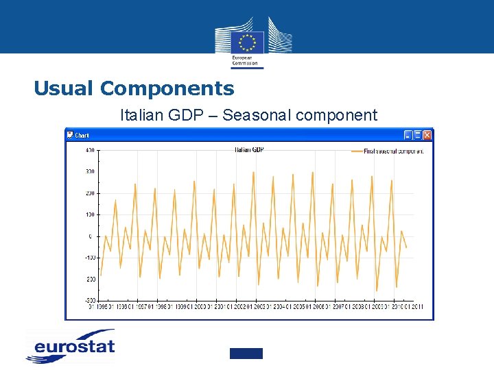
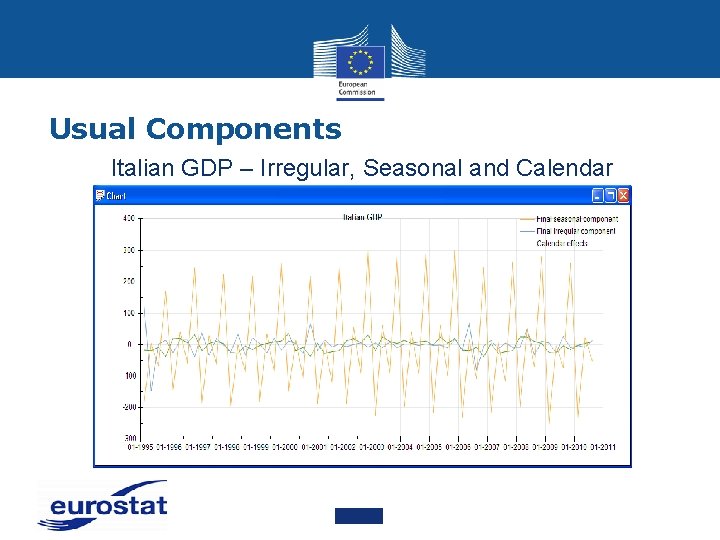
Usual Components • The Trend Component • The Trend is the long term evolution of the series that can be observed on several decades • The Cycle Component • The Cycle is the smooth and quasi-periodic movement of the series that can usually be observed around the long term trend • The Seasonal Component (Seasonality) • Fluctuations observed during the year (each month, each quarter) and which appear to repeat themselves on a more or less regular basis from one year to other

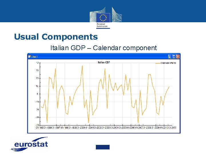
Usual Components • The Calendar Effect • Any economic effect which appears to be related to the calendar (e. g. one more Sunday in the month can affect the production) • The Irregular Component is composed of residual and random fluctuations that cannot be attributed to the other “systematic” components • Outliers • Different kinds of Outliers can be defined • year to other

Usual Components Italian GDP – Trend component

Usual Components Italian GDP – Seasonal component

Usual Components Italian GDP – Calendar component

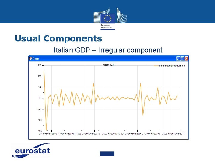
Usual Components Italian GDP – Irregular component

Usual Components Italian GDP – Irregular, Seasonal and Calendar

Trend • The Trend Component is defined as the longterm movement in a series • The Trend is a reflection of the underlying level of the series. This is typically due to influences such as population growth, price inflation and general economic development • The Trend Component is sometimes referred to as the Trend-Cycle (see Cycle Component)

Cause of Seasonality • Seasonality and Climate: due to the variations of the weather and of the climate (seasons!) • Examples: agriculture, consumption of electricity (heating) • Seasonality and Institutions: due to the social habits and practices or to the administrative rules • Examples: effect of Christmas on the retail trade, of the fiscal year on some financial variables, of the academic calendar • Indirect Seasonality: due to the Seasonality that affects other sectors • Examples: toy industry is affected a long time before Christmas. A Seasonal increase in the retail trade has an impact on manufacturing, deliveries, etc. .

Seasonal Adjustment • Seasonal Adjustment is the process of estimating and removing the Seasonal Effects from a Time Series, and by Seasonal we mean an effect that happens at the same time and with the same magnitude and direction every year • The basic goal of Seasonal Adjustment is to decompose a Time Series into several different components, including a Seasonal Component and an Irregular Component • Because the Seasonal effects are an unwanted feature of the Time Series, Seasonal Adjustment can be thought of as focused noise reduction

Seasonal Adjustment • Since Seasonal effects are annual effects, the data must be collected at a frequency less than annually, usually monthly or quarterly • For the data to be useful for Time Series analysis, the data should be comparable over time. This means: • The measurements should be taken over discrete (nonoverlapping) consecutive periods, i. e. , every month or every quarter • The definition of the concept and the way it is measured should be consistent over time

Seasonal Adjustment • Keep in mind that longer series are NOT necessarily better. If the series has changed the way the data is measured or defined, it might be better to cut off the early part of the series to keep the series as homogeneous as possible • The best way to decide if your series needs to be shortened is to investigate the data collection methods and the economic factors associated with your series and choose a length that gives you the most homogeneous series possible

Seasonal Adjustment • During Seasonal Adjustment, we remove Seasonal Effects from the original series. If present, we also remove Calendar Effects. The Seasonally Adjusted series is therefore a combination of the Trend and Irregular Components • One common misconception is that Seasonal Adjustment will also hide any Outliers present. This is not the case. If there is some kind of unusual event, we need that information for analysis, and Outliers are included in the Seasonally Adjusted series

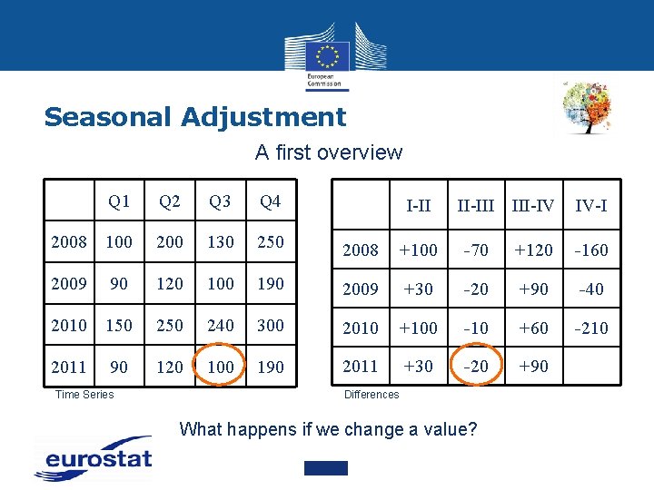
Seasonal Adjustment A first overview Q 1 Q 2 Q 3 Q 4 2008 100 200 130 250 2008 +100 -70 +120 -160 2009 90 120 100 190 2009 +30 -20 +90 -40 2010 150 240 300 2010 +100 -10 +60 -210 2011 90 120 100 190 2011 +30 -20 +90 Time Series I-II II-III III-IV Differences What happens if we change a value? IV-I

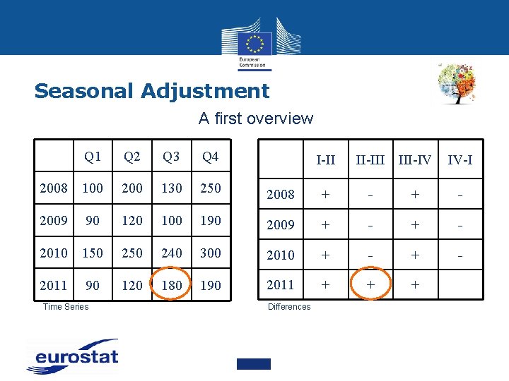
Seasonal Adjustment A first overview Q 1 Q 2 Q 3 Q 4 2008 100 200 130 250 2008 + - 2009 90 120 100 190 2009 + - 2010 150 240 300 2010 + - 2011 90 120 180 190 2011 + + + Time Series I-II Differences II-III III-IV IV-I

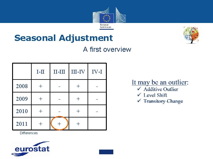
Seasonal Adjustment A first overview I-II II-III III-IV IV-I 2008 + - 2009 + - 2010 + - 2011 + + + Differences

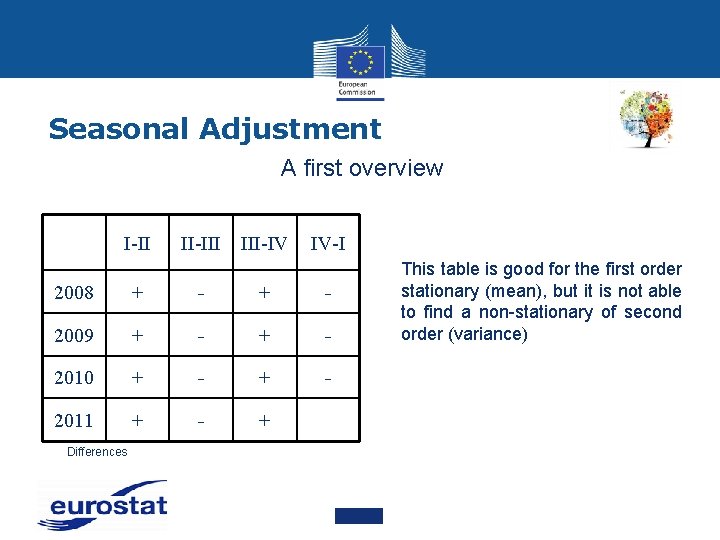
Seasonal Adjustment A first overview I-II II-III III-IV IV-I 2008 + - 2009 + - 2010 + - 2011 + - + Differences This table is good for the first order stationary (mean), but it is not able to find a non-stationary of second order (variance)

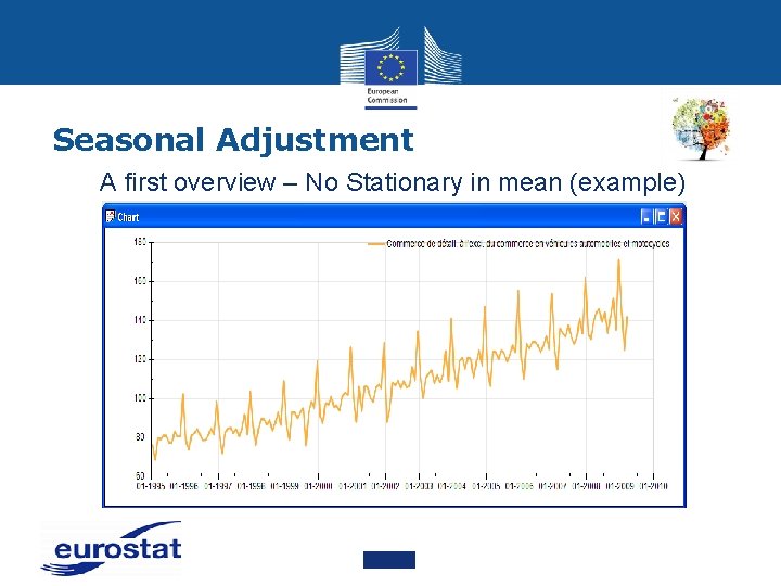
Seasonal Adjustment A first overview – No Stationary in mean (example)

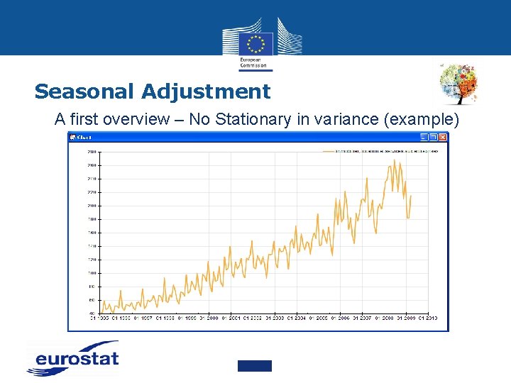
Seasonal Adjustment A first overview – No Stationary in variance (example)

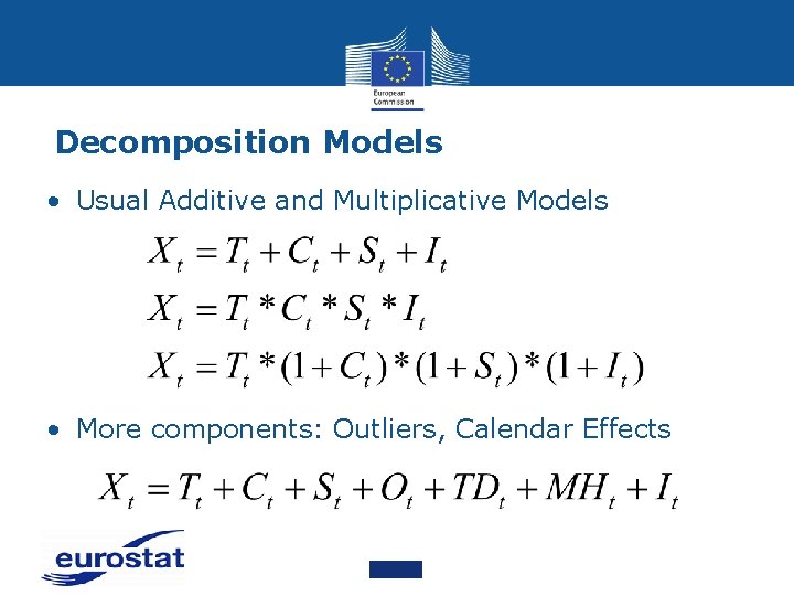
Decomposition Models • Usual Additive and Multiplicative Models • More components: Outliers, Calendar Effects

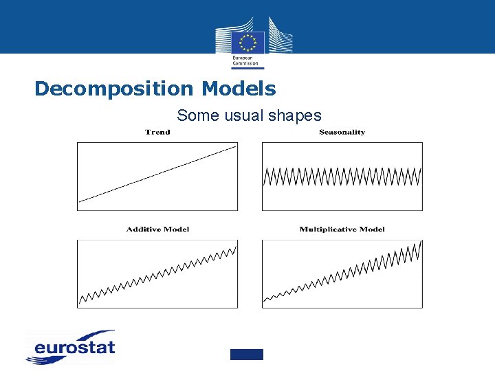
Decomposition Models Some usual shapes

Calendar Adjustment • Calendar Effects typically include: • • Different number of Working Days in a specific period Composition of Working Days Leap Year effect Moving Holidays (Easter, Ramadan, etc. )

Calendar Adjustment - Trading Day Effect • Recurring effects associated with individual days of the week. This occurs because only non-leap-year Februaries have four of each type of day: four Mondays, four Tuesdays, etc. • All other months have an excess of some types of days. If an activity is higher on some days compared to others, then the series can have a Trading Day effect. For example, building permit offices are usually closed on Saturday and Sunday • Thus, the number of building permits issued in a given month is likely to be higher if the month contains a surplus of weekdays and lower if the month contains a surplus of weekend days

Calendar Adjustment - Moving Holiday Effect • Effects from holidays that are not always on the same day of a month, such as Labor Day or Thanksgiving. The most important Moving Holiday in the US and European countries is Easter, not only because it moves between days, but also because it moves between months since it can occur in March or April

Irregular Component • The Irregular Component is the remaining component of the series after the Seasonal and Trend Components have been removed from the original data • For this reason, it is also sometimes referred to as the Residual Component. It attempts to capture the remaining short term fluctuations in the series which are neither systematic nor predictable

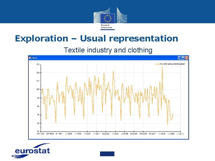
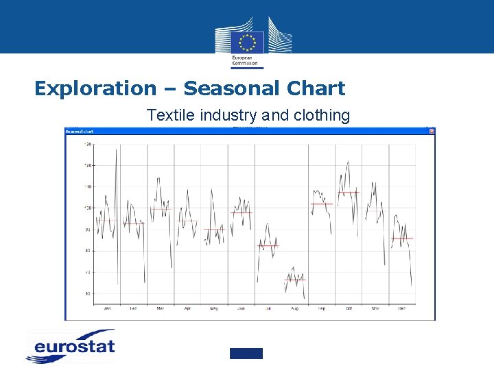
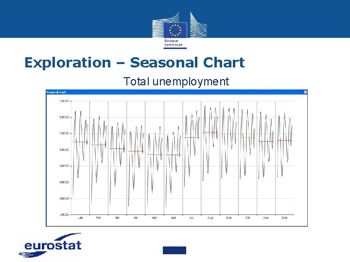
Exploration – Basic tools • Exploration is a very essential step analyzing a Time Series • Looking for “structures” in the series when • Trend, Seasonality, “strange” points or behavior etc. • Helps to formulate a global or decomposition model for the series • Graphics are a key player in this exploration

Exploration – Usual representation Textile industry and clothing

Exploration – Seasonal Chart Textile industry and clothing

Exploration – Seasonal Chart Total unemployment

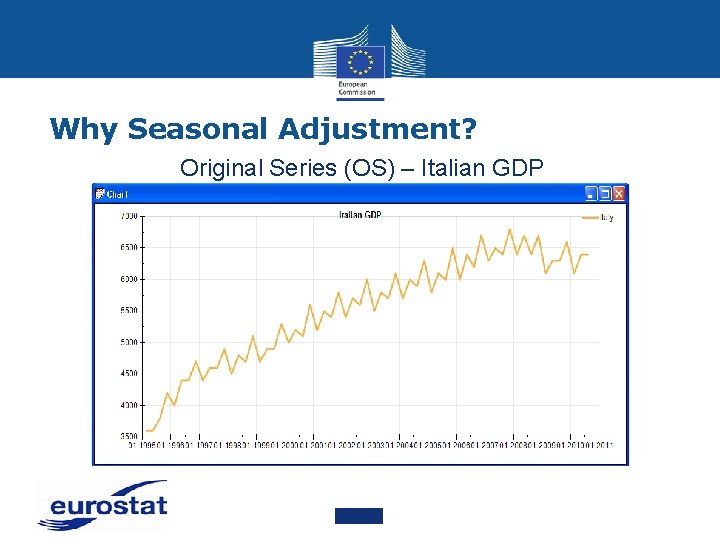
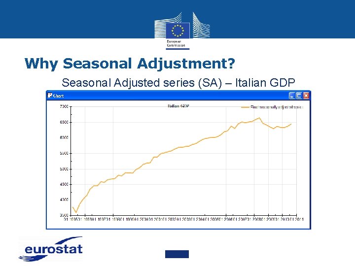
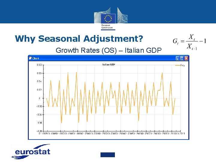
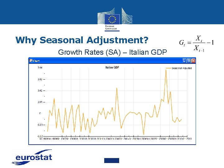
Why Seasonal Adjustment? • Business cycle analysis • To improve comparability: • Over time: o Example: how to compare the first quarter (with February) to the fourth quarter (with Christmas)? • Across space: o Never forget that while we are freezing at work, Australians are burning on the beach! o Very important to compare European national economies (convergence of business cycles) or sectors

Why Seasonal Adjustment? Original Series (OS) – Italian GDP

Why Seasonal Adjustment? Seasonal Adjusted series (SA) – Italian GDP

Why Seasonal Adjustment? Growth Rates (OS) – Italian GDP

Why Seasonal Adjustment? Growth Rates (SA) – Italian GDP

Why Seasonal Adjustment? • The aim of Seasonal Adjustment is to eliminate Seasonal and Calendar Effects. Hence there are no Seasonal and Calendar Effects in a perfectly Seasonally Adjusted series • In other words: Seasonal Adjustment transforms the world we live in into a world where no Seasonal and Calendar Effects occur. In a Seasonally Adjusted world the temperature is exactly the same in winter as in the summer, there are no holidays, Christmas is abolished, people work every day in the week with the same intensity (no break over the weekend), etc.

Step by step procedures for SA • Step 0: Number of observations • It is a requirement for Seasonal Adjustment that the Times Series have to be at least 3 years-long (36 observations) for monthly series and 4 years-long (16 observations) for quarterly series. If a series does not fulfill this condition, it is not long enough for Seasonal Adjustment. Of course these are minimum values, series can be longer for an adequate adjustment or for the computation of diagnostics depending on the fitted ARIMA model

Step by step procedures for SA • Step 1: Graph • • • It is important to have a look at the data and graph of the original Time Series before running a Seasonal Adjustment method Series with possible Outlier values should be identified. Verification is needed concerning that the outliers are valid and there is not sign problem in the data for example captured erroneously The missing observations in the Time Series should be identified and explained. Series with too many missing values will cause estimation problems If series are part of an aggregate series, it should be verified that the starting and ending dates for all component series are the same Look at the Spectral Graph of the Original Series (optional)

Step by step procedures for SA • Step 2: Constant in variance • • • The type of transformation should be used automatically. Confirm the results of the automatic choice by looking at graphs of the series. If the diagnostics for choosing between Additive and Multiplicative decomposition models are inconclusive, then you can chose to continue with the type of transformation used in the past to allow for consistency between years or it is recommended to visually inspect the graph of the series If the series has zero and negative values, then this series must be additively adjusted If the series has a decreasing level with positive values close to zero, then multiplicative adjustment must be used

Step by step procedures for SA • Step 3: Calendar Effects • • • It should be determined which regression effects, such as Trading/Working Day, Leap Year, Moving Holidays (e. g. Easter) and national holidays, are plausible for the series If the effects are not plausible for the series or the coefficients for the effect are not significant, then regressors should not be fit for the effects If the coefficients for the effects are marginally significant, then it should be determined if there is a reason to keep the effects in the model If the automatic test does not indicate the need for Trading Day regressor, but there is a peak at the first trading day frequency of the spectrum of the residuals, then it may fit a Trading Day regressor manually If the series is long enough and the coefficients for the effect are high significant then the six regressors versions of the Trading Day effect should be used instead of one

Step by step procedures for SA • Step 4: Outliers • • There are two possibilities to identify Outliers. The first is when we identify series with possible Outlier values as in STEP 1. If some Outliers are marginally significant, it should be analysed if there is a reason to keep the Outliers in the model. The second possibility is when automatic Outlier correction is used. The results should be confirmed by looking at graphs of the series and any available information (economic, social, etc. ) about the possible cause of the detected Outlier should be used A high number of Outliers signifies that there is a problem related to weak stability of the process, or that there is a problem with the reliability of the data. Series with high number of Outliers relative to the series’ length should be identified. This can result in regression model over-specification. The series should be attempted to re-model with reducing the number of Outliers Those Outlier regressors that might be revised should be considered carefully. Expert information about Outliers is especially important at the end of the series because the types of these Outliers are uncertain from a mathematical point of view and the change of type leads later to large revisions Check from period to period the location of Outliers, because it should be not always the same

Step by step procedures for SA • Step 5: ARIMA model • • Automatic model identification should be used once a year, but the re-estimation the parameters are recommended when new observation appends. If the results are not plausible the following procedure is advisable. High-order ARIMA model coefficients that are not significant should be identified. It can be helpful to simplify the model by reducing the order of the model, taking care not to skip lags of AR models. For Moving Average (MA) models, it is not necessary to skip model lags whose coefficients are not significant. Before choosing an MA model with skipped lag, the full-order MA model should be fitted and skip a lag only if that lag’s model coefficient is not significantly different from zero The BIC and AIC statistics should be looked at in order to confirm the global quality of fit statistics

Step by step procedures for SA • Step 6: Check the filter (optional) • • The critical X-11 options in X-12 ARIMA are the options that control the extreme value procedure in the X-11 module and the Trend Filters and Seasonal Filters used for Seasonal Adjustment Verify that the Seasonal Filters are in agreement generally with the global moving Seasonality ratio After reviewing the Seasonal Filter choices, the Seasonal Filters in the input file should be set to the specific chosen length so they will not change during the production The SI-ratio Graphs in the X-12 ARIMA output file should be looked at. Any month with many extreme values relative to the length of the time series should be identified. This may be needed for raising the sigma limits for the extreme value procedure

Step by step procedures for SA • Step 7: Residuals • • There should not be any residual Seasonal and Calendar Effects in the published Seasonally Adjusted series or in the Irregular Component The spectral graph of the Seasonally Adjusted series and the Irregular Component should be looked at (optional). If there is residual Seasonality or Calendar Effect, as indicated by the spectral peaks, the model and regressor options should be checked in order to remove residual peaks If the series is a composite indirect adjustment of several component series, the checks mentioned above in aggregation approach should be performed Among others the diagnostics of normality and Ljung-Box Qstatistics should be looked at in order to check the residuals of the model

Step by step procedures for SA • Step 8: Diagnostic • The stability diagnostics for Seasonal Adjustment are the sliding spans and revision history. Large revisions and instability indicated by the history and sliding spans diagnostics show that the Seasonal Adjustment is not useful

Step by step procedures for SA • Step 9: Publication policy • A reference paper with the quality report (if it is available) should be issued once a year as a separate publication which has to include the following information: 1. The Seasonal Adjustment method in use 2. The decision rules for the choice of different options in the program 3. The aggregation policy 4. The Outlier detection and correction methods 5. The decision rules for transformation 6. The revision policy 7. The description of the Working/Trading Day adjustment 8. The contact address

day 2, morning • Identification of types of Outliers • Additive outlier • Transitory change • Level shift • Calendar Effect and its determinants • Trading days • Moving holidays • X-13 ARIMA vs. Tramo/Seats • How to use the ESS guidelines on SA

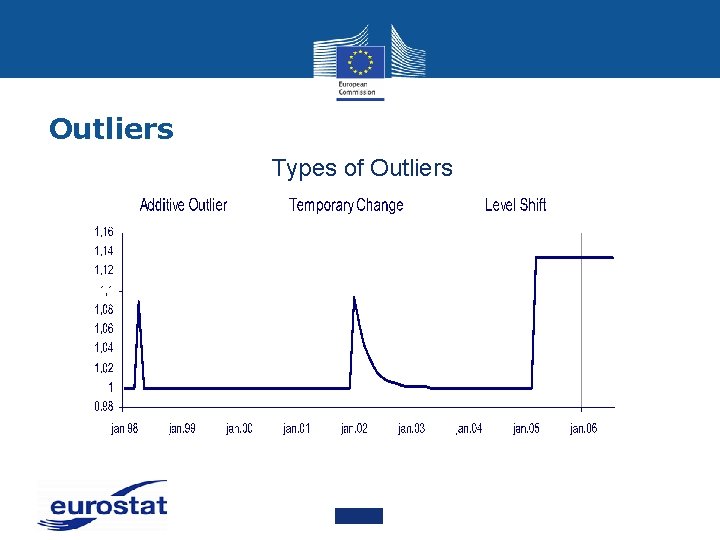
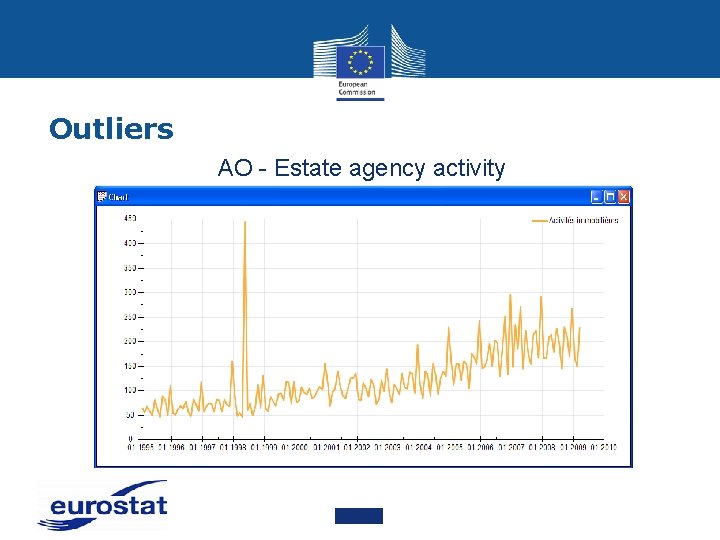
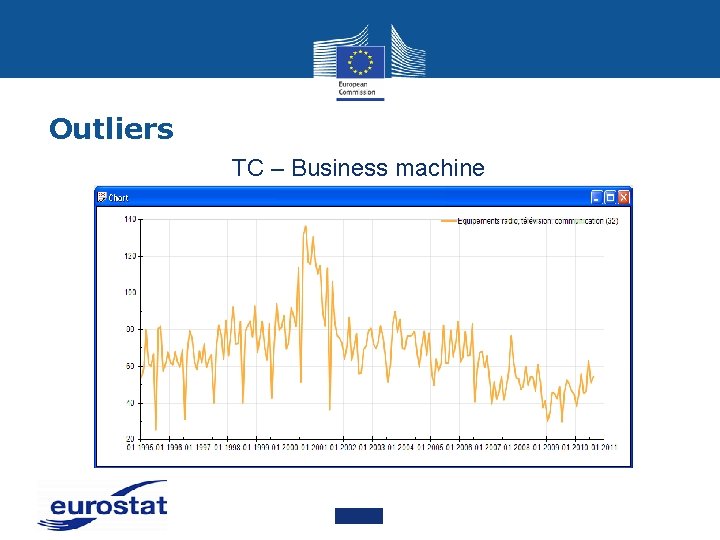
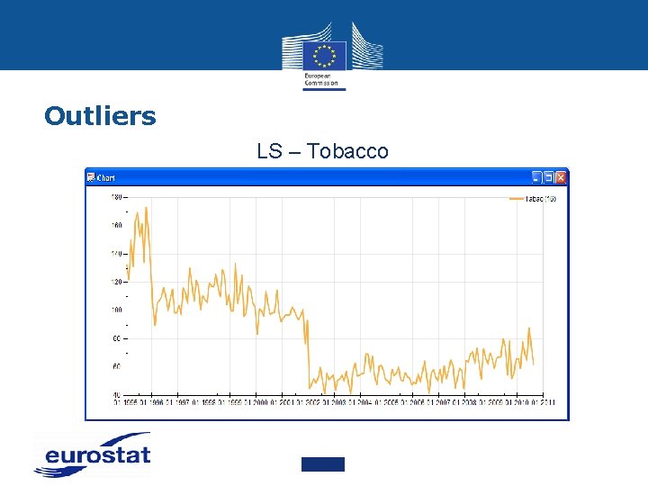
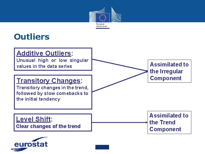
Outliers • Outliers are data which do not fit in the tendency of the Time Series observed, which fall outside the range expected on the basis of the typical pattern of the Trend and Seasonal Components • Additive Outlier (AO): the value of only one observation is affected. AO may either be caused by random effects or due to an identifiable cause as a strike, bad weather or war • Temporary Change (TC): the value of one observation is extremely high or low, then the size of the deviation reduces gradually (exponentially) in the course of the subsequent observations until the Time Series returns to the initial level • Level Shift (LS): starting from a given time period, the level of the Time Series undergoes a permanent change. Causes could include: change in concepts and definitions of the survey population, in the collection method, in the economic behavior, in the legislation or in the social traditions

Outliers Types of Outliers

Outliers AO - Estate agency activity

Outliers TC – Business machine

Outliers LS – Tobacco

Outliers Additive Outliers: Unusual high or low singular values in the data series Transitory Changes: Assimilated to the Irregular Component Transitory changes in the trend, followed by slow comebacks to the initial tendency Level Shift: Clear changes of the trend Assimilated to the Trend Component

Outliers • The smoothness of series can be decided by statisticians and the policy must be defined in advance • Consult the users • This choice can influence dramatically the credibility • Outliers in last quarter are very difficult to be identified • Some suggestions: • Look at the growth rates • Conduct a continuous analysis of external sources to identify reasons of Outliers • Where possible always add an economic explanation • Be transparent (LS, AO, TC)

Calendar Effects • Time Series: usually a daily activity measured on a monthly or quarterly basis only • Flow: monthly or quarterly sum of the observed variable • Stock: the variable is observed at a precise date (example: first or last day of the month) • Some movements in the series are due to the variation in the calendar from a period to another • Can especially be observed in flow series • Example: the production for a month often depends on the number of days

Calendar Effects • Trading Day Effect • Can be observed in production activities or retail sale • Trading Days (Working Days) = days usually worked according to the business uses • Often these days are non-public holiday weekdays (Monday, Tuesday, Wednesday, Thursday, Friday) • Production usually increases with the number of working days in the month

Calendar Effects • “Day of the week” effect • Example: Retail sale turnover is likely to be more important on Saturdays than on other weekdays • Statutory (Public) Holidays and Moving Holidays • Most of statutory holidays are linked to a date, not to a day of the week (Christmas) • Some holidays can move across the year (Easter, Ramadan) and their effect is not completely seasonal • Months and quarters are not equivalent and not directly comparable

X-13 ARIMA VS TRAMO/SEATS • Seasonal Adjustment is usually done with an off-the-shelf program. Three popular tools are: • X-13 ARIMA (Census Bureau) • TRAMO/SEATS (Bank of Spain) • JDEMETRA+ (Eurostat), interface X-13 ARIMA and Tramo/Seats • X-13 ARIMA is Filter based: always estimate a Seasonal Component and remove it from the series even if no Seasonality is present, but not all the estimates of the Seasonally Adjusted series will be good • TRAMO/SEATS is model based: method variants of decomposition of Time Series into non-observed components

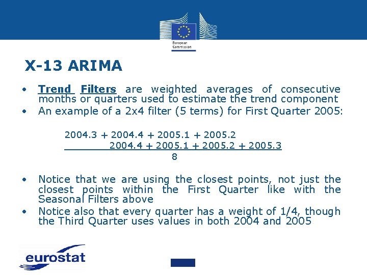
X-13 ARIMA • • • A Filter is a weighted average where the weights sum to 1 Seasonal Filters are the filters used to estimate the Seasonal Component. Ideally, Seasonal Filters are computed using values from the same month or quarter (for example an estimate for January would come from a weighted average of the surrounding Januaries) The Seasonal Filters available in X-13 ARIMA consist of seasonal Moving Averages of consecutive values within a given month or quarter. An n x m Moving Average is an m-term simple average taken over n consecutive sequential spans

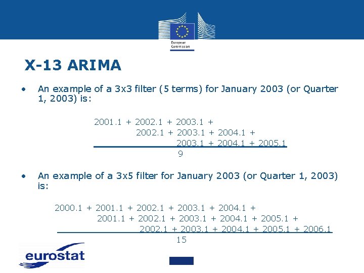
X-13 ARIMA • An example of a 3 x 3 filter (5 terms) for January 2003 (or Quarter 1, 2003) is: 2001. 1 + 2002. 1 + 2003. 1 + 2004. 1 + 2005. 1 9 • An example of a 3 x 5 filter for January 2003 (or Quarter 1, 2003) is: 2000. 1 + 2001. 1 + 2002. 1 + 2003. 1 + 2004. 1 + 2005. 1 + 2006. 1 15

X-13 ARIMA • • Trend Filters are weighted averages of consecutive months or quarters used to estimate the trend component An example of a 2 x 4 filter (5 terms) for First Quarter 2005: 2004. 3 + 2004. 4 + 2005. 1 + 2005. 2 + 2005. 3 8 • • Notice that we are using the closest points, not just the closest points within the First Quarter like with the Seasonal Filters above Notice also that every quarter has a weight of 1/4, though the Third Quarter uses values in both 2004 and 2005

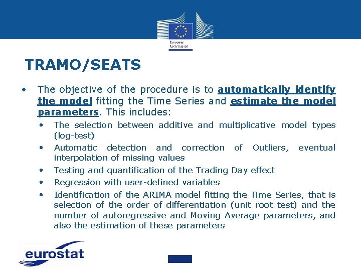
TRAMO/SEATS • The objective of the procedure is to automatically identify the model fitting the Time Series and estimate the model parameters. This includes: • • • The selection between additive and multiplicative model types (log-test) Automatic detection and correction of Outliers, eventual interpolation of missing values Testing and quantification of the Trading Day effect Regression with user-defined variables Identification of the ARIMA model fitting the Time Series, that is selection of the order of differentiation (unit root test) and the number of autoregressive and Moving Average parameters, and also the estimation of these parameters

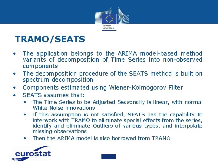
TRAMO/SEATS • • The application belongs to the ARIMA model-based method variants of decomposition of Time Series into non-observed components The decomposition procedure of the SEATS method is built on spectrum decomposition Components estimated using Wiener-Kolmogorov Filter SEATS assumes that: • • • The Time Series to be Adjusted Seasonally is linear, with normal White Noise innovations If this assumption is not satisfied, SEATS has the capability to interwork with TRAMO to eliminate special effects from the series, identify and eliminate Outliers of various types, and interpolate missing observations Then the ARIMA model is also borrowed from TRAMO

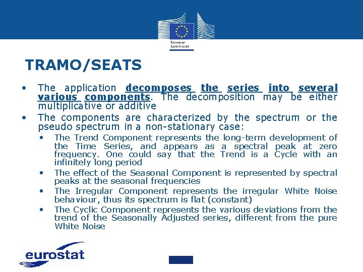
TRAMO/SEATS • • The application decomposes the series into several various components. The decomposition may be either multiplicative or additive The components are characterized by the spectrum or the pseudo spectrum in a non-stationary case: • • The Trend Component represents the long-term development of the Time Series, and appears as a spectral peak at zero frequency. One could say that the Trend is a Cycle with an infinitely long period The effect of the Seasonal Component is represented by spectral peaks at the seasonal frequencies The Irregular Component represents the irregular White Noise behaviour, thus its spectrum is flat (constant) The Cyclic Component represents the various deviations from the trend of the Seasonally Adjusted series, different from the pure White Noise

TRAMO/SEATS • • First SEATS decomposes the ARIMA model of the Time Series observed, that is, identifies the ARIMA models of the components. This operation takes place in the frequency domain. The spectrum is divided into the sum of the spectra related to the various components Actually SEATS decides on the basis of the argument of roots, which is mostly located near to the frequency of the spectral peak • The roots of high absolute value related to 0 frequency are assigned • • • to the Trend Component The roots related to the seasonal frequencies to the Seasonal Component The roots of low absolute value related to 0 frequency and the Cyclic (between 0 and the first Seasonal frequency) and those related to frequencies between the Seasonal ones are assigned to the Cyclic Component The Irregular Component is always deemed as white noise

ESS Guidelines on SA • Introduced in 2009 and revised in 2015 • Chapters subdivided into specific items describing different steps of the SA process • Items presented in a standard structure providing: 1. Description of the issue 2. List of options which could be followed to perform the step 3. Prioritized list of three alternatives from most recommended one to the one to avoid (A, B and C) 4. Concise list of main references • Added value: 1. Conceptual framework and practical implementation steps 2. Both for experienced users and beginners

Historical background • Since early nineties: • Informal group on Seasonal Adjustment • Stocktaking exercise: • BV 4, Dainties, SABL, Census family (X-11, X-12 ARIMA etc. ), TRAMO/SEATS • Criteria (among others): • Estimation of a Calendar Component • Treatment of Outliers • Statistical tests • Long and controversial discussions: • At the end preference for X-12 -ARIMA and TRAMO/SEATS

Historical background • EUROSTAT developed DEMETRA+ in order to support comparisons between X-12 -ARIMA and TRAMO/SEATS • ECB/EUROSTAT Seasonal Adjustment Steering Group was founded to promote further harmonization • After the EUROSTAT crises, the work on the Guidelines started • 2008: Agreement on the guidelines of the CMFB and the SPC • 2012: The National Bank of Belgium in collaboration with EUROSTAT developed JDEMETRA+, an open source tool for SA • 2012 -2013: Task Force for the revision of the ESS Guidelines on SA, final version published in May 2015

JDEMETRA+ • JDEMETRA+ is not only a user-friendly graphical interface, comparable with DEMETRA+, but also a set of open Java libraries that can be used to deal with time series related issues • JDEMETRA+ is built around the concepts and the algorithms used in the two leading SA methods, i. e. TRAMO/SEATS and X-12 ARIMA / X-13 ARIMA SEATS • The algorithms have been reengineered, following an objectoriented approach, that allows for easier handling, extensions or modifications • X-13 ARIMA SEATS includes a module that uses the ARIMA model based seasonal adjustment procedure from the SEATS seasonal adjustment program

Questions?