Seasonal Adjustment and DEMETRA ESTP course EUROSTAT 3

Seasonal Adjustment and DEMETRA+ ESTP course EUROSTAT 3 – 5 May 2011 Dario Buono and Enrico Infante Unit B 2 – Research and Methodology © 2011 by EUROSTAT. All rights reserved. Open to the public 04/05/2011

Session 2 – May 4 th Identification of type of Outliers Calendar Effects and its determinants Moving Averages X-12 ARIMA and TRAMO/SEATS 04/05/2011 ESTP course Dario Buono, Enrico Infante 2

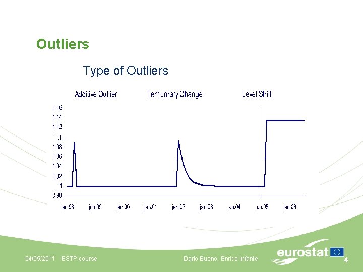
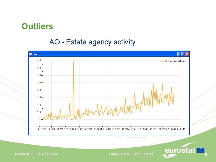
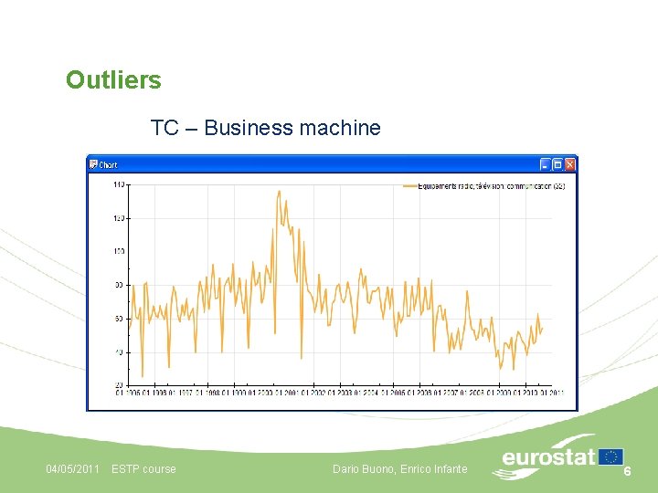
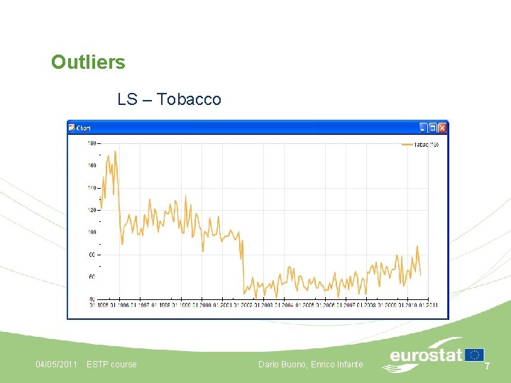
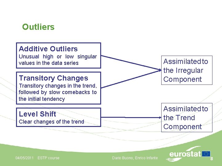
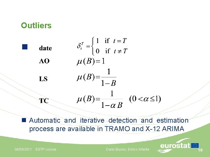
Outliers n Outliers are data which do not fit in the tendency of the Time Series observed, which fall outside the range expected on the basis of the typical pattern of the Trend and Seasonal Components n Additive Outlier (AO): the value of only one observation is affected. AO may either be caused by random effects or due to an identifiable cause as a strike, bad weather or war n Temporary Change (TC): the value of one observation is extremely high or low, then the size of the deviation reduces gradually (exponentially) in the course of the subsequent observations until the Time Series returns to the initial level n Level Shift (LS): starting from a given time period, the level of the Time Series undergoes a permanent change. Causes could include: change in concepts and definitions of the survey population, in the collection method, in the economic behavior, in the legislation or in the social traditions 04/05/2011 ESTP course Dario Buono, Enrico Infante 3

Outliers Type of Outliers 04/05/2011 ESTP course Dario Buono, Enrico Infante 4

Outliers AO - Estate agency activity 04/05/2011 ESTP course Dario Buono, Enrico Infante 5

Outliers TC – Business machine 04/05/2011 ESTP course Dario Buono, Enrico Infante 6

Outliers LS – Tobacco 04/05/2011 ESTP course Dario Buono, Enrico Infante 7

Outliers Additive Outliers Unusual high or low singular values in the data series Assimilated to the Irregular Component Transitory Changes Transitory changes in the trend, followed by slow comebacks to the initial tendency Assimilated to the Trend Component Level Shift Clear changes of the trend 04/05/2011 ESTP course Dario Buono, Enrico Infante 8

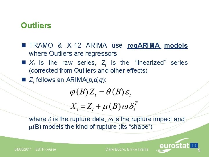
Outliers n TRAMO & X-12 ARIMA use reg. ARIMA models where Outliers are regressors n Xt is the raw series, Zt is the “linearized” series (corrected from Outliers and other effects) n Zt follows an ARIMA(p, d, q): where is the rupture date, is the rupture impact and (B) models the kind of rupture (its “shape”) 04/05/2011 ESTP course Dario Buono, Enrico Infante 9

Outliers n n Automatic and iterative detection and estimation process are available in TRAMO and X-12 ARIMA 04/05/2011 ESTP course Dario Buono, Enrico Infante 10

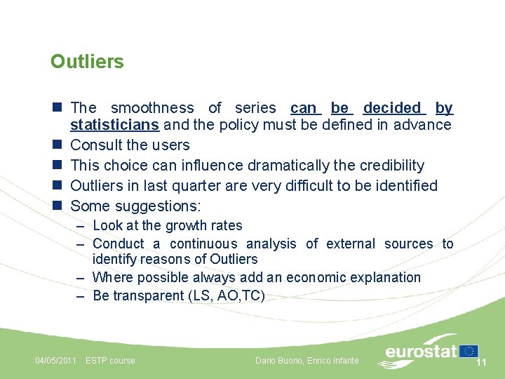
Outliers n The smoothness of series can be decided by statisticians and the policy must be defined in advance n Consult the users n This choice can influence dramatically the credibility n Outliers in last quarter are very difficult to be identified n Some suggestions: – Look at the growth rates – Conduct a continuous analysis of external sources to identify reasons of Outliers – Where possible always add an economic explanation – Be transparent (LS, AO, TC) 04/05/2011 ESTP course Dario Buono, Enrico Infante 11

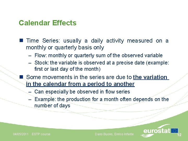
Calendar Effects n Time Series: usually a daily activity measured on a monthly or quarterly basis only – Flow: monthly or quarterly sum of the observed variable – Stock: the variable is observed at a precise date (example: first or last day of the month) n Some movements in the series are due to the variation in the calendar from a period to another – Can especially be observed in flow series – Example: the production for a month often depends on the number of days 04/05/2011 ESTP course Dario Buono, Enrico Infante 12

Calendar Effects n Trading Day Effect – Can be observed in production activities or retail sale – Trading Days (Working Days) = days usually worked according to the business uses – Often these days are non public holiday weekdays (Monday, Tuesday, Wednesday, Thursday, Friday) – Production usually increases with the number of working days in the month 04/05/2011 ESTP course Dario Buono, Enrico Infante 13

Calendar Effects n “Day of the week” effect – Example: Retail sale turnover is likely to be more important on Saturdays than on other weekdays n Statutory (Public) Holidays and Moving Holidays – Most of statutory holidays are linked to a date, not to a day of the week (Christmas) – Some holidays can move across the year (Easter, Ramadan) and their effect is not completely seasonal n Months and quarters are not equivalent and not directly comparables 04/05/2011 ESTP course Dario Buono, Enrico Infante 14

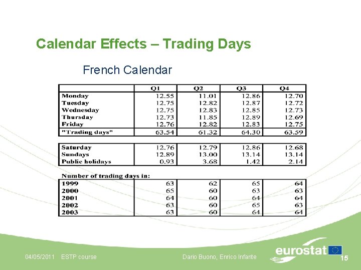
Calendar Effects – Trading Days French Calendar 04/05/2011 ESTP course Dario Buono, Enrico Infante 15

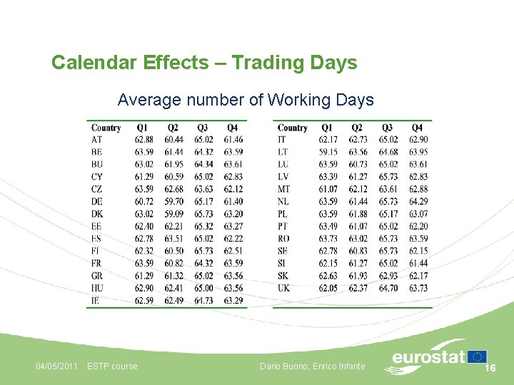
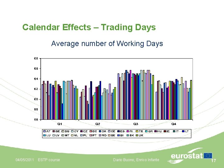
Calendar Effects – Trading Days Average number of Working Days 04/05/2011 ESTP course Dario Buono, Enrico Infante 16

Calendar Effects – Trading Days Average number of Working Days 04/05/2011 ESTP course Dario Buono, Enrico Infante 17

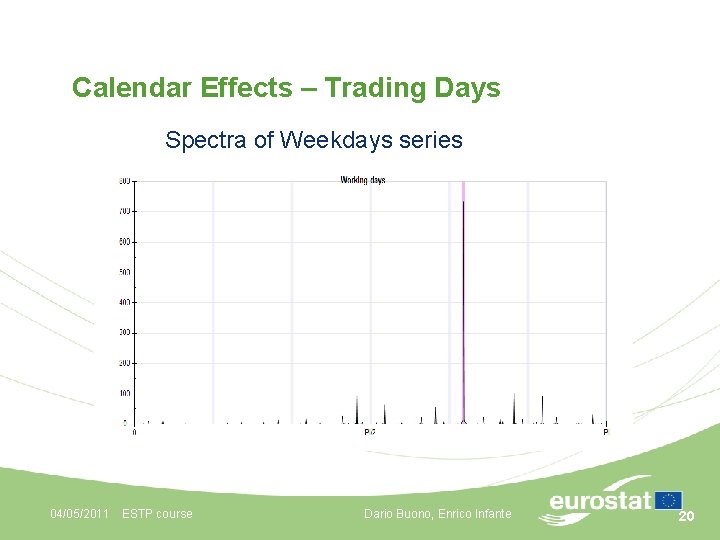
Calendar Effects – Trading Days n Calendar Effects can be partly considered seasonal: – The number of Trading Days is almost always smaller in February than in March – Some months may have more public holidays (ex: May in France), and therefore less trading days than others n Thus, we can: – Either estimate the non seasonal Calendar Effects – Make the correction of both Seasonal and Calendar Effects n Spectra of the “Weekday” series: number of Mondays, Tuesdays, …, Friday per month 04/05/2011 ESTP course Dario Buono, Enrico Infante 18

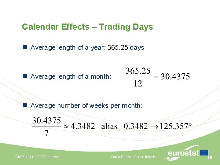
Calendar Effects – Trading Days n Average length of a year: 365. 25 days n Average length of a month: n Average number of weeks per month: 04/05/2011 ESTP course Dario Buono, Enrico Infante 19

Calendar Effects – Trading Days Spectra of Weekdays series 04/05/2011 ESTP course Dario Buono, Enrico Infante 20

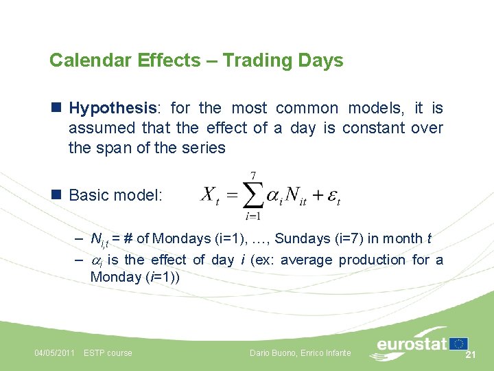
Calendar Effects – Trading Days n Hypothesis: for the most common models, it is assumed that the effect of a day is constant over the span of the series n Basic model: – Ni, t = # of Mondays (i=1), …, Sundays (i=7) in month t – i is the effect of day i (ex: average production for a Monday (i=1)) 04/05/2011 ESTP course Dario Buono, Enrico Infante 21

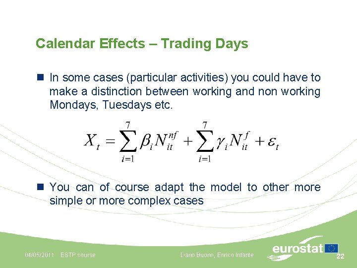
Calendar Effects – Trading Days n In some cases (particular activities) you could have to make a distinction between working and non working Mondays, Tuesdays etc. n You can of course adapt the model to other more simple or more complex cases 04/05/2011 ESTP course Dario Buono, Enrico Infante 22

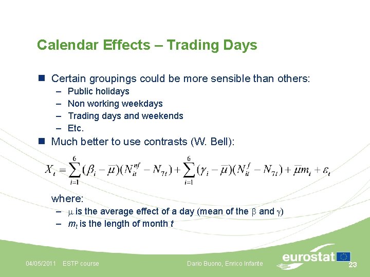
Calendar Effects – Trading Days n Certain groupings could be more sensible than others: – – Public holidays Non working weekdays Trading days and weekends Etc. n Much better to use contrasts (W. Bell): where: – is the average effect of a day (mean of the and ) – mt is the length of month t 04/05/2011 ESTP course Dario Buono, Enrico Infante 23

Calendar Effects – Trading Days n The variables take into account a part of Seasonality: the length of the month is seasonal, the White Monday is always a Monday etc. n If we want to estimate the non seasonal Calendar Effects, we can remove from the variables their longterm average n In this case, the explanatory variables do not have any Trend or Seasonality. Thus, the dependant variable must be stationary, an Irregular Component for example (X 11), or a reg. ARIMA model should be used n X-12 ARIMA and TRAMO-SEATS 04/05/2011 ESTP course Dario Buono, Enrico Infante 24

Coffee-Break!!! We will restart in 15 minutes 04/05/2011 ESTP course Dario Buono, Enrico Infante 25

Calendar Effects – Moving Holidays n The date of some public holidays (usually religious events) moves across the year and can affect different months or quarters according to the year n Examples: Ramadan, Chinese New Year, Easter (Catholic or Orthodox) etc. n The effect of the event could be gradual and could affect the days before or after the event itself: Chocolate sales around Easter n We focus in the following on the treatment of Easter but the methodology and the models can be easily adapted 04/05/2011 ESTP course Dario Buono, Enrico Infante 26

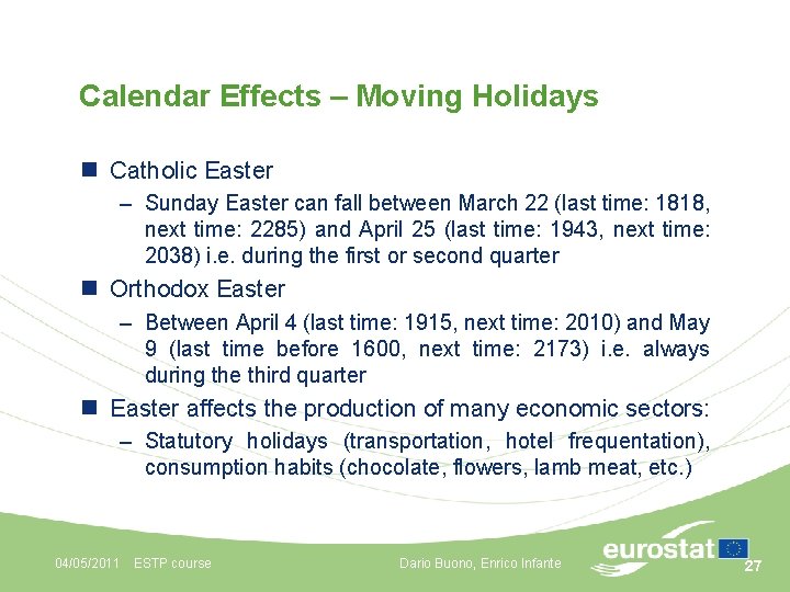
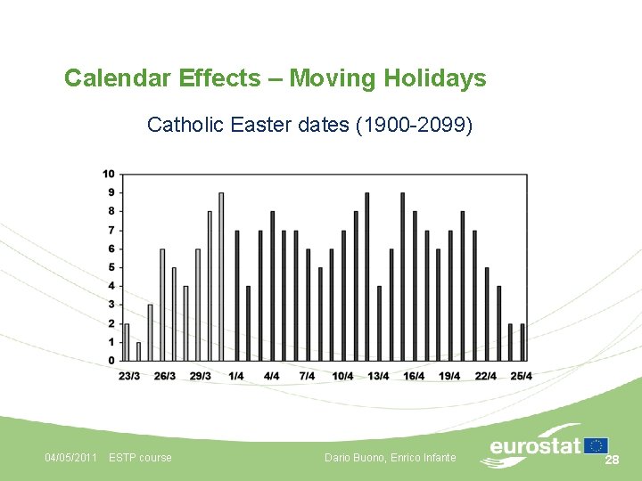
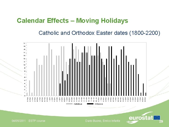
Calendar Effects – Moving Holidays n Catholic Easter – Sunday Easter can fall between March 22 (last time: 1818, next time: 2285) and April 25 (last time: 1943, next time: 2038) i. e. during the first or second quarter n Orthodox Easter – Between April 4 (last time: 1915, next time: 2010) and May 9 (last time before 1600, next time: 2173) i. e. always during the third quarter n Easter affects the production of many economic sectors: – Statutory holidays (transportation, hotel frequentation), consumption habits (chocolate, flowers, lamb meat, etc. ) 04/05/2011 ESTP course Dario Buono, Enrico Infante 27

Calendar Effects – Moving Holidays Catholic Easter dates (1900 -2099) 04/05/2011 ESTP course Dario Buono, Enrico Infante 28

Calendar Effects – Moving Holidays Catholic and Orthodox Easter dates (1800 -2200) 04/05/2011 ESTP course Dario Buono, Enrico Infante 29

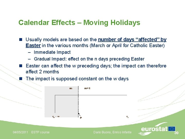
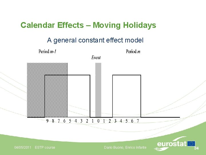
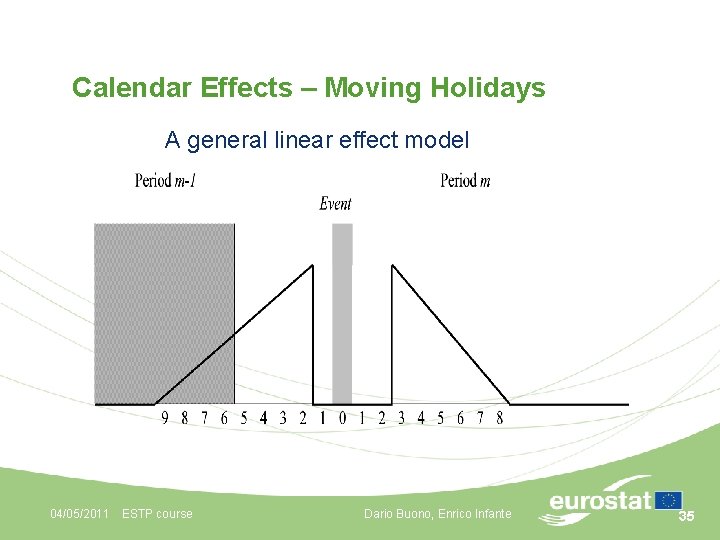
Calendar Effects – Moving Holidays n Usually models are based on the number of days “affected” by Easter in the various months (March or April for Catholic Easter) – Immediate Impact – Gradual Impact: effect on the n days preceding Easter n Easter can affect the w preceding days; the impact can therefore affect 2 months n The impact is supposed constant on the w days 04/05/2011 ESTP course Dario Buono, Enrico Infante 30

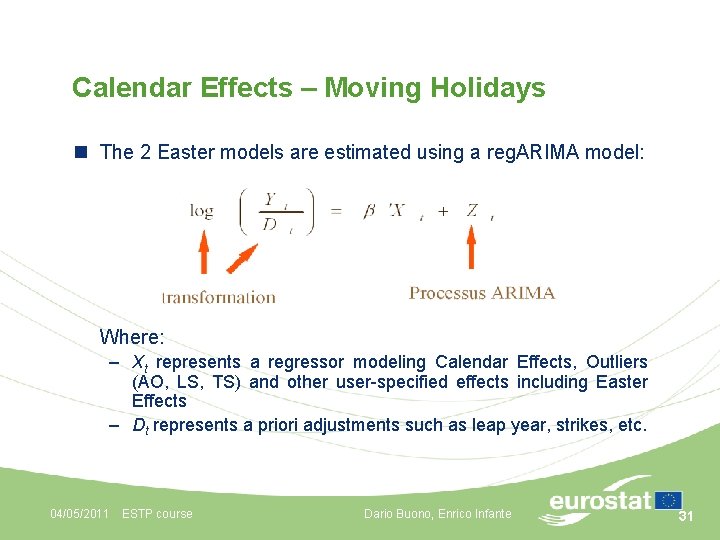
Calendar Effects – Moving Holidays n The 2 Easter models are estimated using a reg. ARIMA model: Where: – Xt represents a regressor modeling Calendar Effects, Outliers (AO, LS, TS) and other user-specified effects including Easter Effects – Dt represents a priori adjustments such as leap year, strikes, etc. 04/05/2011 ESTP course Dario Buono, Enrico Infante 31

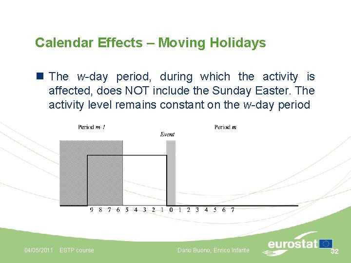
Calendar Effects – Moving Holidays n The w-day period, during which the activity is affected, does NOT include the Sunday Easter. The activity level remains constant on the w-day period 04/05/2011 ESTP course Dario Buono, Enrico Infante 32

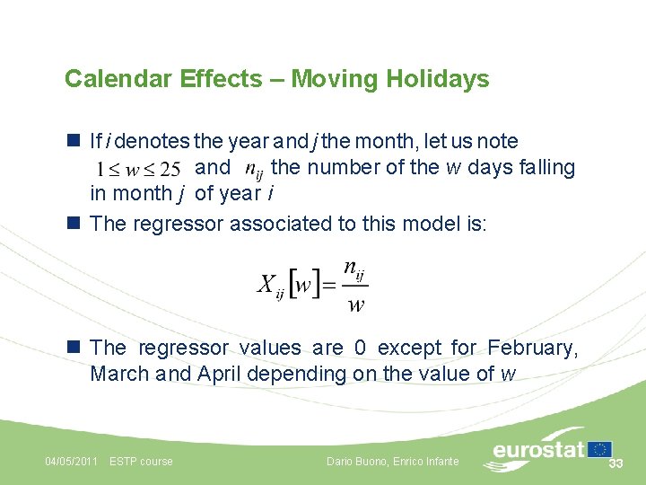
Calendar Effects – Moving Holidays n If i denotes the year and j the month, let us note and the number of the w days falling in month j of year i n The regressor associated to this model is: n The regressor values are 0 except for February, March and April depending on the value of w 04/05/2011 ESTP course Dario Buono, Enrico Infante 33

Calendar Effects – Moving Holidays A general constant effect model 04/05/2011 ESTP course Dario Buono, Enrico Infante 34

Calendar Effects – Moving Holidays A general linear effect model 04/05/2011 ESTP course Dario Buono, Enrico Infante 35

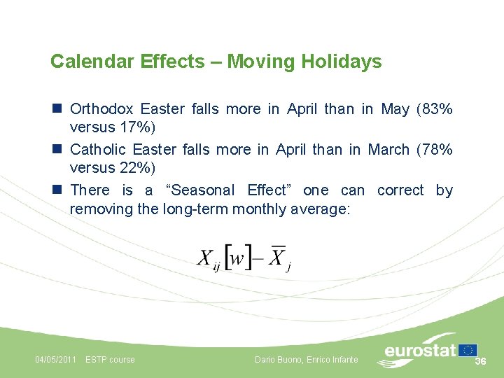
Calendar Effects – Moving Holidays n Orthodox Easter falls more in April than in May (83% versus 17%) n Catholic Easter falls more in April than in March (78% versus 22%) n There is a “Seasonal Effect” one can correct by removing the long-term monthly average: 04/05/2011 ESTP course Dario Buono, Enrico Infante 36

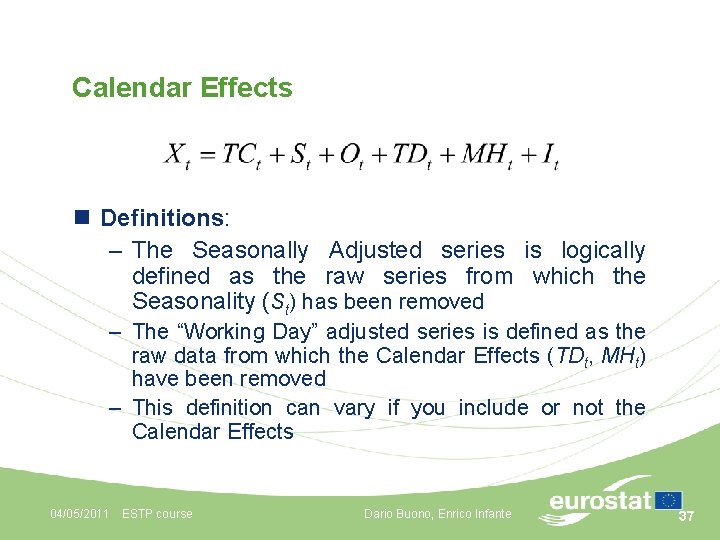
Calendar Effects n Definitions: – The Seasonally Adjusted series is logically defined as the raw series from which the Seasonality (St) has been removed – The “Working Day” adjusted series is defined as the raw data from which the Calendar Effects (TDt, MHt) have been removed – This definition can vary if you include or not the Calendar Effects 04/05/2011 ESTP course Dario Buono, Enrico Infante 37

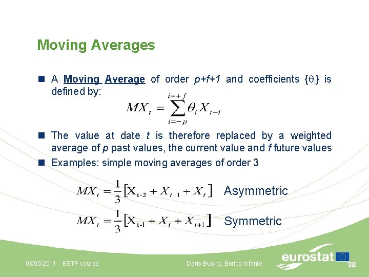
Moving Averages n A Moving Average of order p+f+1 and coefficients { i} is defined by: n The value at date t is therefore replaced by a weighted average of p past values, the current value and f future values n Examples: simple moving averages of order 3 Asymmetric Symmetric 03/05/2011 ESTP course Dario Buono, Enrico Infante 38

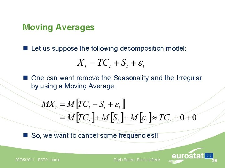
Moving Averages n Let us suppose the following decomposition model: n One can want remove the Seasonality and the Irregular by using a Moving Average: n So, we want to cancel some frequencies!! 03/05/2011 ESTP course Dario Buono, Enrico Infante 39

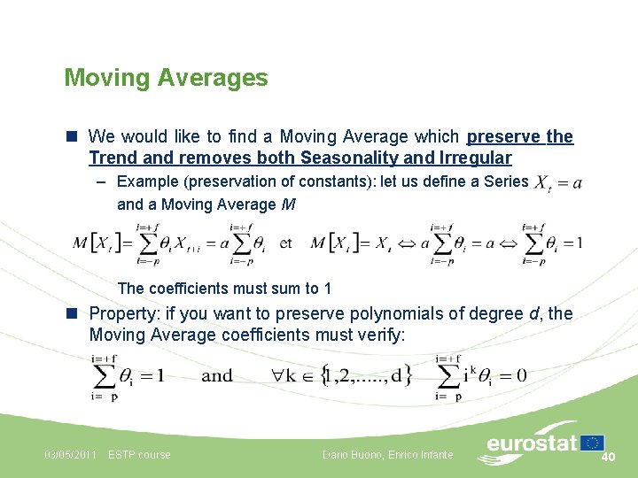
Moving Averages n We would like to find a Moving Average which preserve the Trend and removes both Seasonality and Irregular – Example (preservation of constants): let us define a Series and a Moving Average M The coefficients must sum to 1 n Property: if you want to preserve polynomials of degree d, the Moving Average coefficients must verify: 03/05/2011 ESTP course Dario Buono, Enrico Infante 40

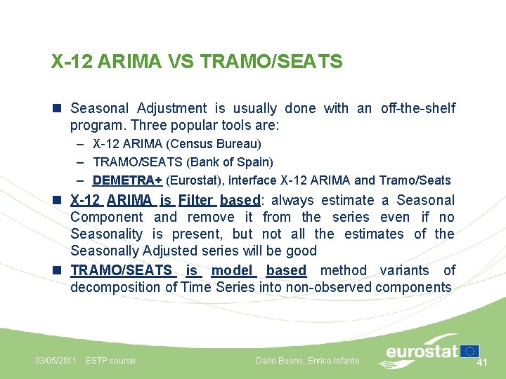
X-12 ARIMA VS TRAMO/SEATS n Seasonal Adjustment is usually done with an off-the-shelf program. Three popular tools are: – X-12 ARIMA (Census Bureau) – TRAMO/SEATS (Bank of Spain) – DEMETRA+ (Eurostat), interface X-12 ARIMA and Tramo/Seats n X-12 ARIMA is Filter based: always estimate a Seasonal Component and remove it from the series even if no Seasonality is present, but not all the estimates of the Seasonally Adjusted series will be good n TRAMO/SEATS is model based method variants of decomposition of Time Series into non-observed components 03/05/2011 ESTP course Dario Buono, Enrico Infante 41

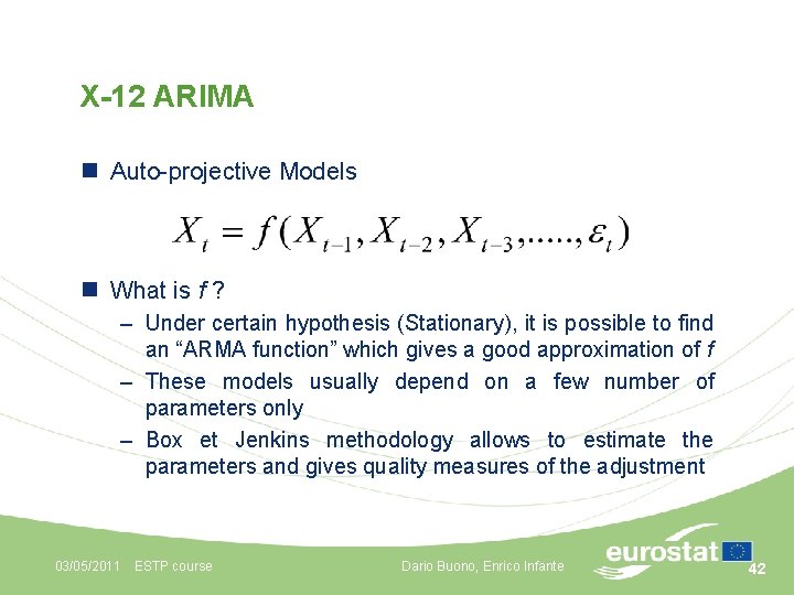
X-12 ARIMA n Auto-projective Models n What is f ? – Under certain hypothesis (Stationary), it is possible to find an “ARMA function” which gives a good approximation of f – These models usually depend on a few number of parameters only – Box et Jenkins methodology allows to estimate the parameters and gives quality measures of the adjustment 03/05/2011 ESTP course Dario Buono, Enrico Infante 42

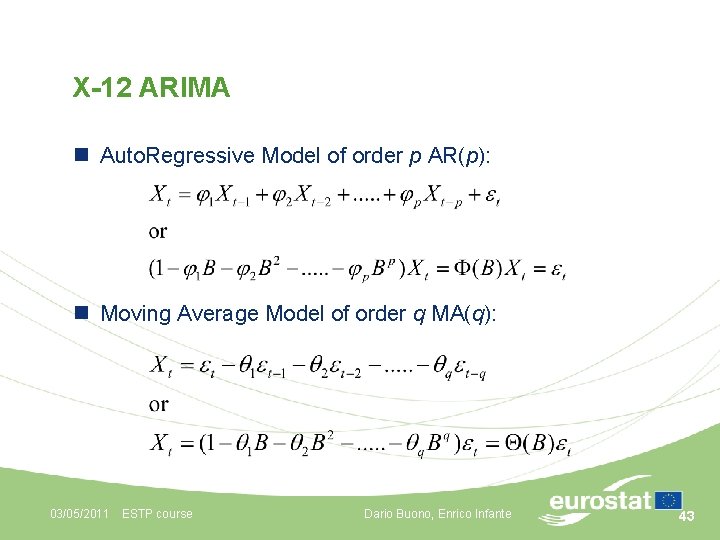
X-12 ARIMA n Auto. Regressive Model of order p AR(p): n Moving Average Model of order q MA(q): 03/05/2011 ESTP course Dario Buono, Enrico Infante 43

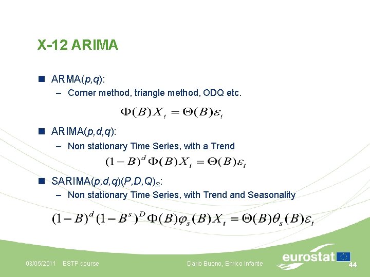
X-12 ARIMA n ARMA(p, q): – Corner method, triangle method, ODQ etc. n ARIMA(p, d, q): – Non stationary Time Series, with a Trend n SARIMA(p, d, q)(P, D, Q)S: – Non stationary Time Series, with Trend and Seasonality 03/05/2011 ESTP course Dario Buono, Enrico Infante 44

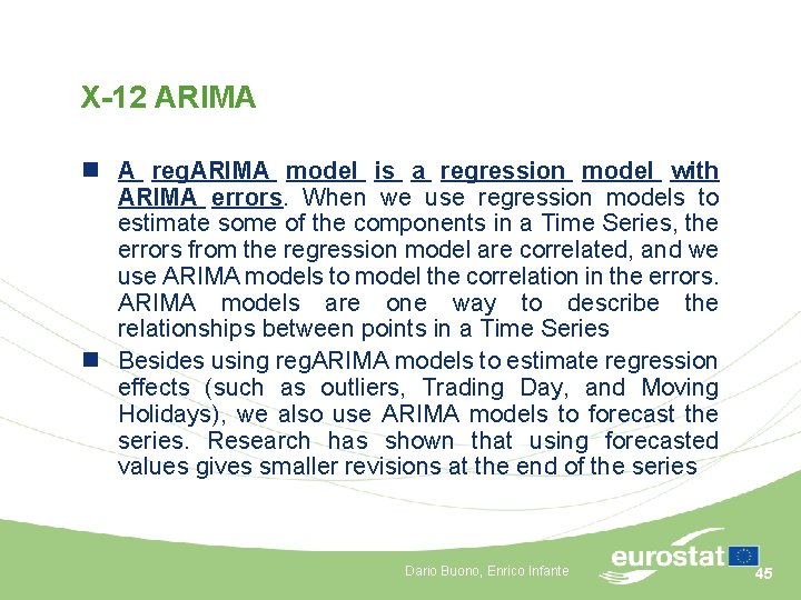
X-12 ARIMA n A reg. ARIMA model is a regression model with ARIMA errors. When we use regression models to estimate some of the components in a Time Series, the errors from the regression model are correlated, and we use ARIMA models to model the correlation in the errors. ARIMA models are one way to describe the relationships between points in a Time Series n Besides using reg. ARIMA models to estimate regression effects (such as outliers, Trading Day, and Moving Holidays), we also use ARIMA models to forecast the series. Research has shown that using forecasted values gives smaller revisions at the end of the series Dario Buono, Enrico Infante 45

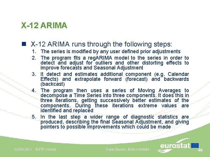
X-12 ARIMA n X-12 ARIMA runs through the following steps: 1. The series is modified by any user defined prior adjustments 2. The program fits a reg. ARIMA model to the series in order to detect and adjust for outliers and other distorting effects to improve forecasts and Seasonal Adjustment 3. It detect and estimates additional component (e. g. Calendar Effects) and extrapolate forward (forecast) and backwards (backcast) 4. The program then uses a series of Moving Averages to decompose a Time Series into three components. It does this in three iterations, getting successively better estimates of the components. During these iterations extreme values are identified and replaced 5. In the last step a wider range of diagnostic statistics are produced, describing the final Seasonal Adjustment, and giving pointers to possible improvements which could be made 03/05/2011 ESTP course Dario Buono, Enrico Infante 46

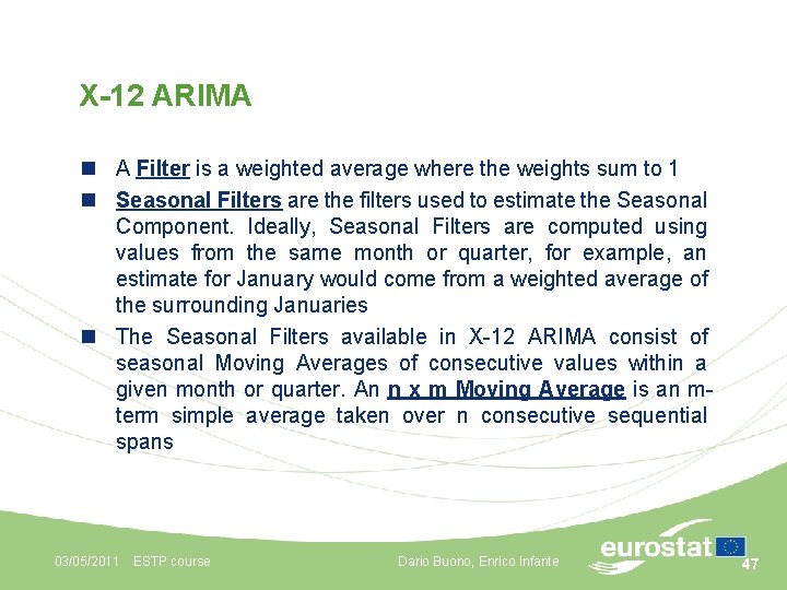
X-12 ARIMA n A Filter is a weighted average where the weights sum to 1 n Seasonal Filters are the filters used to estimate the Seasonal Component. Ideally, Seasonal Filters are computed using values from the same month or quarter, for example, an estimate for January would come from a weighted average of the surrounding Januaries n The Seasonal Filters available in X-12 ARIMA consist of seasonal Moving Averages of consecutive values within a given month or quarter. An n x m Moving Average is an mterm simple average taken over n consecutive sequential spans 03/05/2011 ESTP course Dario Buono, Enrico Infante 47

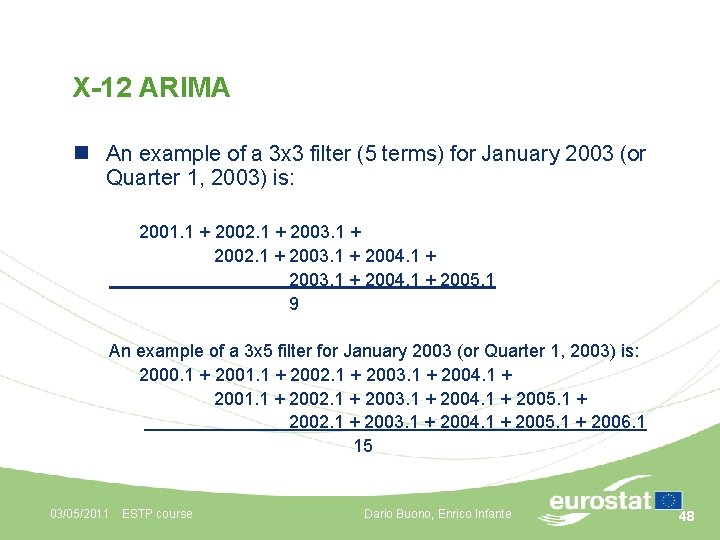
X-12 ARIMA n An example of a 3 x 3 filter (5 terms) for January 2003 (or Quarter 1, 2003) is: 2001. 1 + 2002. 1 + 2003. 1 + 2004. 1 + 2005. 1 9 An example of a 3 x 5 filter for January 2003 (or Quarter 1, 2003) is: 2000. 1 + 2001. 1 + 2002. 1 + 2003. 1 + 2004. 1 + 2005. 1 + 2006. 1 15 03/05/2011 ESTP course Dario Buono, Enrico Infante 48

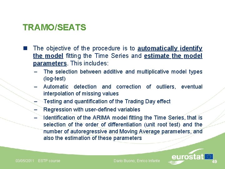
TRAMO/SEATS n The objective of the procedure is to automatically identify the model fitting the Time Series and estimate the model parameters. This includes: – – – The selection between additive and multiplicative model types (log-test) Automatic detection and correction of outliers, eventual interpolation of missing values Testing and quantification of the Trading Day effect Regression with user-defined variables Identification of the ARIMA model fitting the Time Series, that is selection of the order of differentiation (unit root test) and the number of autoregressive and Moving Average parameters, and also the estimation of these parameters 03/05/2011 ESTP course Dario Buono, Enrico Infante 49

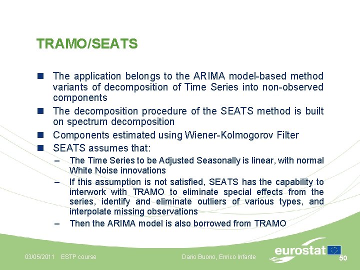
TRAMO/SEATS n The application belongs to the ARIMA model-based method variants of decomposition of Time Series into non-observed components n The decomposition procedure of the SEATS method is built on spectrum decomposition n Components estimated using Wiener-Kolmogorov Filter n SEATS assumes that: – – – The Time Series to be Adjusted Seasonally is linear, with normal White Noise innovations If this assumption is not satisfied, SEATS has the capability to interwork with TRAMO to eliminate special effects from the series, identify and eliminate outliers of various types, and interpolate missing observations Then the ARIMA model is also borrowed from TRAMO 03/05/2011 ESTP course Dario Buono, Enrico Infante 50

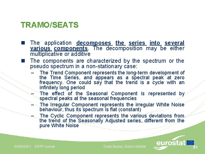
TRAMO/SEATS n The application decomposes the series into several various components. The decomposition may be either multiplicative or additive n The components are characterized by the spectrum or the pseudo spectrum in a non-stationary case: – – The Trend Component represents the long-term development of the Time Series, and appears as a spectral peak at zero frequency. One could say that the trend is a cycle with an infinitely long period The effect of the Seasonal Component is represented by spectral peaks at the seasonal frequencies The Irregular Component represents the irregular White Noise behaviour, thus its spectrum is flat (constant) The Cyclic Component represents the various deviations from the trend of the Seasonally Adjusted series, different from the pure White Noise 03/05/2011 ESTP course Dario Buono, Enrico Infante 51

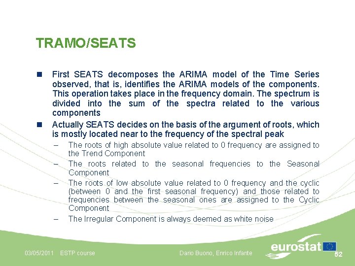
TRAMO/SEATS n n First SEATS decomposes the ARIMA model of the Time Series observed, that is, identifies the ARIMA models of the components. This operation takes place in the frequency domain. The spectrum is divided into the sum of the spectra related to the various components Actually SEATS decides on the basis of the argument of roots, which is mostly located near to the frequency of the spectral peak – – The roots of high absolute value related to 0 frequency are assigned to the Trend Component The roots related to the seasonal frequencies to the Seasonal Component The roots of low absolute value related to 0 frequency and the cyclic (between 0 and the first seasonal frequency) and those related to frequencies between the seasonal ones are assigned to the Cyclic Component The Irregular Component is always deemed as white noise 03/05/2011 ESTP course Dario Buono, Enrico Infante 52

Questions? 04/05/2011 ESTP course Dario Buono, Enrico Infante 53