Course Title Production and Operations Management Course Code

Course Title: Production and Operations Management Course Code: MGT 362 Course Book: Operations Management 10 th Edition. By Jay Heizer & Barry Render 4 -1

Chapter 4: Forecasting 4 -2

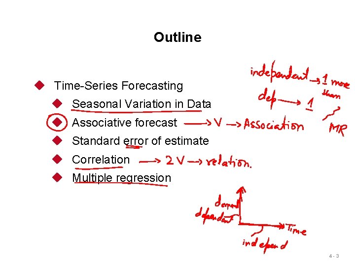
Outline u Time-Series Forecasting u Seasonal Variation in Data u Associative forecast u Standard error of estimate u Correlation u Multiple regression 4 -3

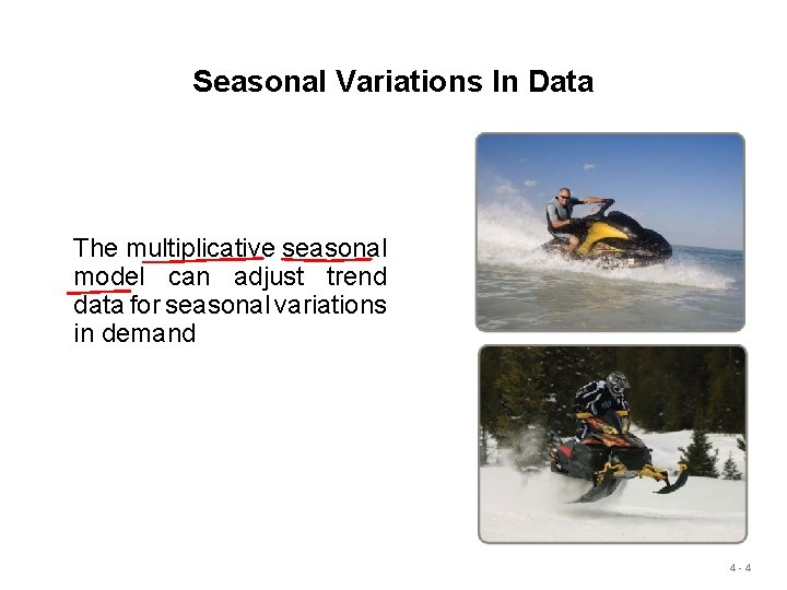
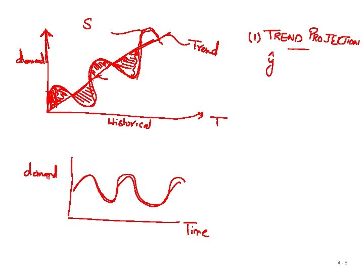
Seasonal Variations In Data The multiplicative seasonal model can adjust trend data for seasonal variations in demand 4 -4

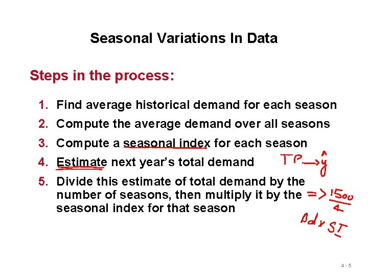
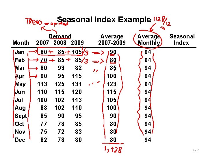
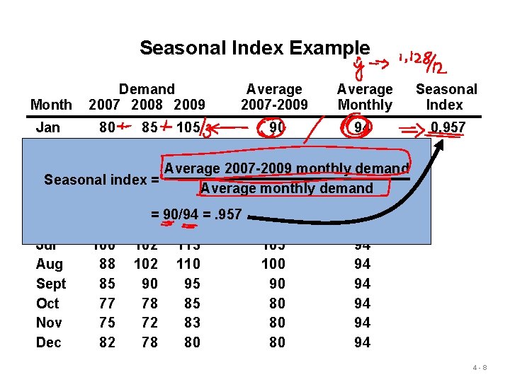
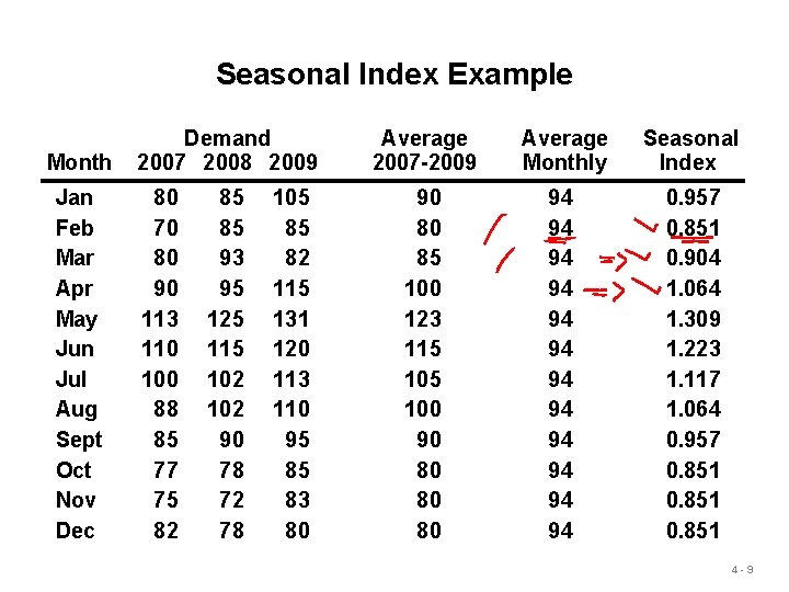
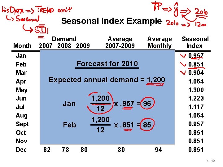
Seasonal Variations In Data Steps in the process: 1. Find average historical demand for each season 2. Compute the average demand over all seasons 3. Compute a seasonal index for each season 4. Estimate next year’s total demand 5. Divide this estimate of total demand by the number of seasons, then multiply it by the seasonal index for that season 4 -5

4 -6

Seasonal Index Example Month Jan Feb Mar Apr May Jun Jul Aug Sept Oct Nov Dec Demand 2007 2008 2009 80 70 80 90 113 110 100 88 85 77 75 82 85 85 93 95 125 115 102 90 78 72 78 105 85 82 115 131 120 113 110 95 85 83 80 Average 2007 -2009 Average Monthly 90 80 85 100 123 115 100 90 80 80 80 94 94 94 Seasonal Index 4 -7

Seasonal Index Example Month Demand 2007 2008 2009 Average 2007 -2009 Average Monthly Jan 80 85 105 90 94 Feb 70 85 85 80 94 Mar 80 93 Average 82 85 monthly 94 2007 -2009 demand Seasonal 90 index 95= 115 Apr 100 94 Average monthly demand May 113 125 131 123 94 = 90/94 =. 957 Jun 110 115 120 115 94 Jul 100 102 113 105 94 Aug 88 102 110 100 94 Sept 85 90 94 Oct 77 78 85 80 94 Nov 75 72 83 80 94 Dec 82 78 80 80 94 Seasonal Index 0. 957 4 -8

Seasonal Index Example Month Jan Feb Mar Apr May Jun Jul Aug Sept Oct Nov Dec Demand 2007 2008 2009 80 70 80 90 113 110 100 88 85 77 75 82 85 85 93 95 125 115 102 90 78 72 78 105 85 82 115 131 120 113 110 95 85 83 80 Average 2007 -2009 Average Monthly Seasonal Index 90 80 85 100 123 115 100 90 80 80 80 94 94 94 0. 957 0. 851 0. 904 1. 064 1. 309 1. 223 1. 117 1. 064 0. 957 0. 851 4 -9

Seasonal Index Example Month Jan Feb Mar Apr May Jun Jul Aug Sept Oct Nov Dec Demand 2007 2008 2009 Average 2007 -2009 Average Monthly 80 85 105 90 94 for 802010 70 85 Forecast 85 94 80 93 82 85 94 annual demand = 1, 200 90 Expected 95 115 100 94 113 125 131 123 94 110 115 120 1, 200 115 94 Jan 113 x. 957 = 96 94 100 102 105 12 88 102 110 100 94 1, 200 85 90 Feb 95 x 90. 851 = 85 94 77 78 85 12 80 94 75 72 83 80 94 82 78 80 80 94 Seasonal Index 0. 957 0. 851 0. 904 1. 064 1. 309 1. 223 1. 117 1. 064 0. 957 0. 851 4 - 10

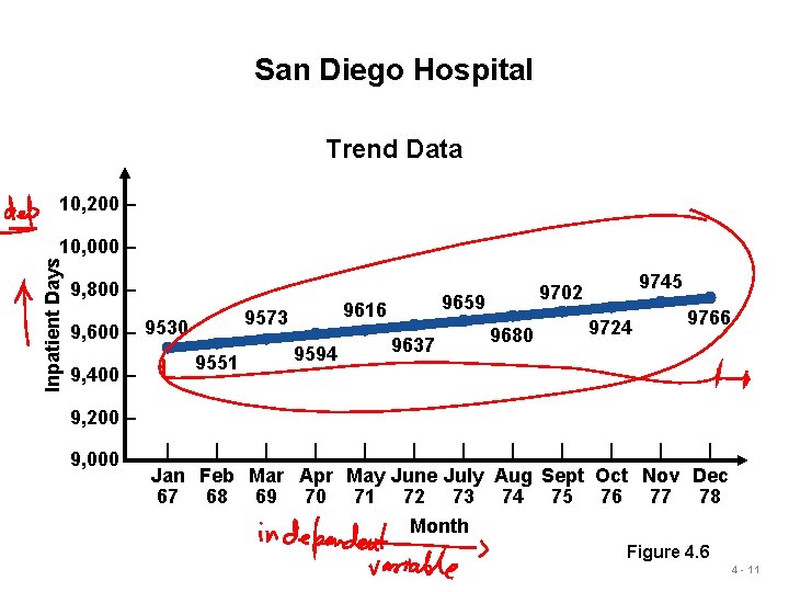
San Diego Hospital Trend Data 10, 200 – Inpatient Days 10, 000 – 9, 800 – 9573 9, 600 – 9530 9, 400 – 9551 9659 9616 9594 9637 9745 9702 9680 9724 9766 9, 200 – 9, 000 – | | | Jan Feb Mar Apr May June July Aug Sept Oct Nov Dec 67 68 69 70 71 72 73 74 75 76 77 78 Month Figure 4. 6 4 - 11

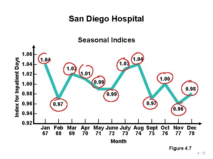
San Diego Hospital Index for Inpatient Days Seasonal Indices 1. 06 – 1. 04 1. 02 – 1. 01 1. 00 0. 99 1. 00 – 0. 98 – 0. 96 – 1. 03 0. 98 0. 99 0. 97 0. 94 – 0. 92 – 1. 04 0. 96 | | | Jan Feb Mar Apr May June July Aug Sept Oct Nov Dec 67 68 69 70 71 72 73 74 75 76 77 78 Month Figure 4. 7 4 - 12

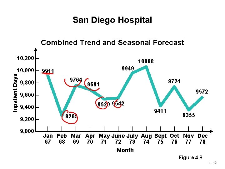
San Diego Hospital Combined Trend and Seasonal Forecast 10, 200 – 10068 9949 Inpatient Days 10, 000 – 9911 9, 800 – 9764 9724 9691 9572 9, 600 – 9520 9542 9, 400 – 9, 200 – 9, 000 – 9411 9265 9355 | | | Jan Feb Mar Apr May June July Aug Sept Oct Nov Dec 67 68 69 70 71 72 73 74 75 76 77 78 Month Figure 4. 8 4 - 13

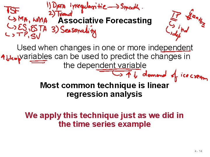
Associative Forecasting Used when changes in one or more independent variables can be used to predict the changes in the dependent variable Most common technique is linear regression analysis We apply this technique just as we did in the time series example 4 - 14

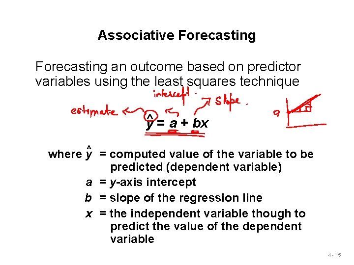
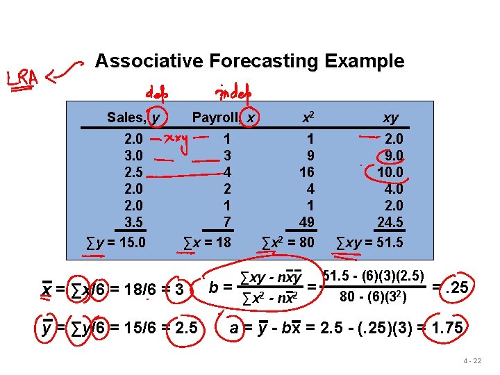
Associative Forecasting an outcome based on predictor variables using the least squares technique y^ = a + bx where y^ = computed value of the variable to be predicted (dependent variable) a = y-axis intercept b = slope of the regression line x = the independent variable though to predict the value of the dependent variable 4 - 15

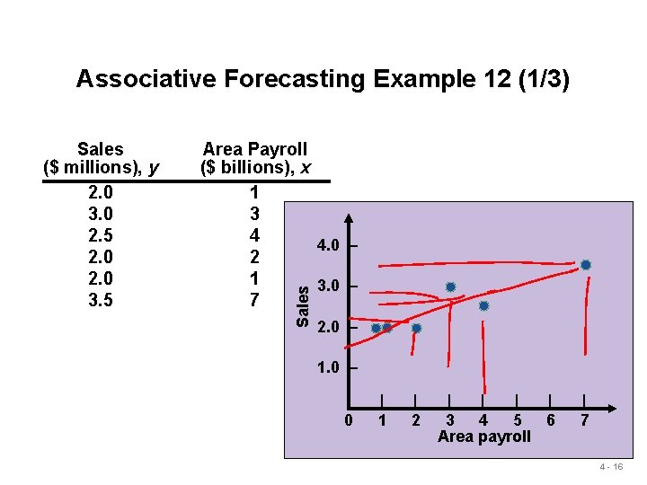
Associative Forecasting Example 12 (1/3) Area Payroll ($ billions), x 1 3 4 4. 0 – 2 1 3. 0 – 7 Sales ($ millions), y 2. 0 3. 0 2. 5 2. 0 3. 5 2. 0 – 1. 0 – 0 | 1 | 2 | | 3 4 5 6 Area payroll | 7 4 - 16

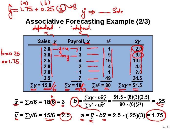
Associative Forecasting Example (2/3) Sales, y 2. 0 3. 0 2. 5 2. 0 3. 5 ∑y = 15. 0 Payroll, x 1 3 4 2 1 7 ∑x = 18 x = ∑x/6 = 18/6 = 3 y = ∑y/6 = 15/6 = 2. 5 b= x 2 1 9 16 4 1 49 ∑x 2 = 80 ∑xy - nxy ∑x 2 - nx 2 = xy 2. 0 9. 0 10. 0 4. 0 24. 5 ∑xy = 51. 5 - (6)(3)(2. 5) 80 - (6)(32) =. 25 a = y - bx = 2. 5 - (. 25)(3) = 1. 75 4 - 17

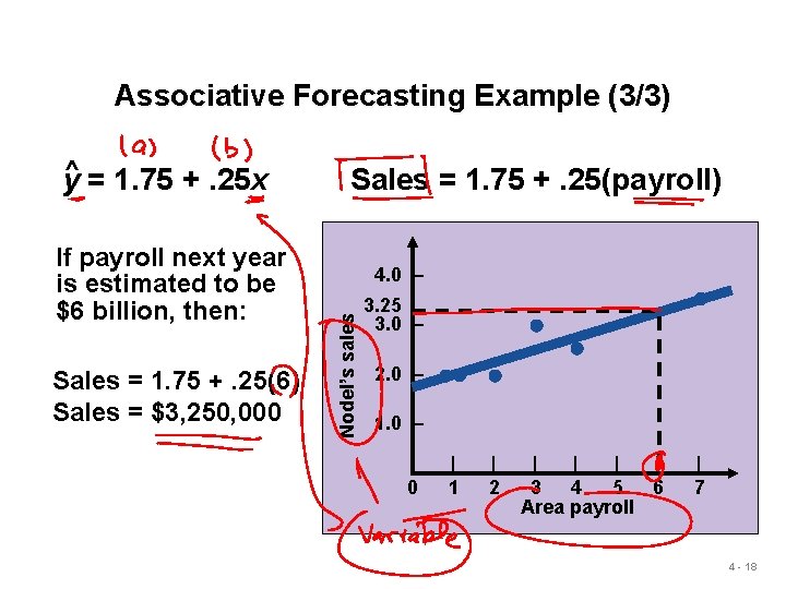
Associative Forecasting Example (3/3) If payroll next year is estimated to be $6 billion, then: Sales = 1. 75 +. 25(6) Sales = $3, 250, 000 Sales = 1. 75 +. 25(payroll) 4. 0 – Nodel’s sales y^ = 1. 75 +. 25 x 3. 25 3. 0 – 2. 0 – 1. 0 – 0 | 1 | 2 | | 3 4 5 6 Area payroll | 7 4 - 18

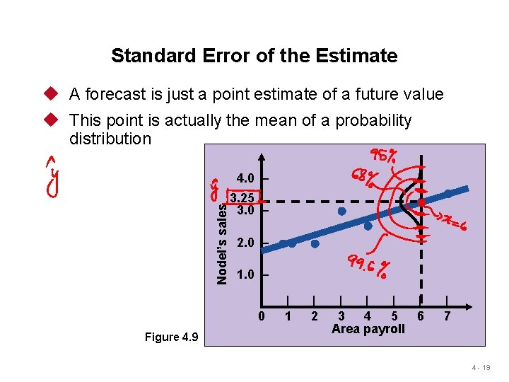
Standard Error of the Estimate u A forecast is just a point estimate of a future value u This point is actually the mean of a probability distribution Nodel’s sales 4. 0 – 3. 25 3. 0 – 2. 0 – 1. 0 – 0 Figure 4. 9 | 1 | 2 | | 3 4 5 6 Area payroll | 7 4 - 19

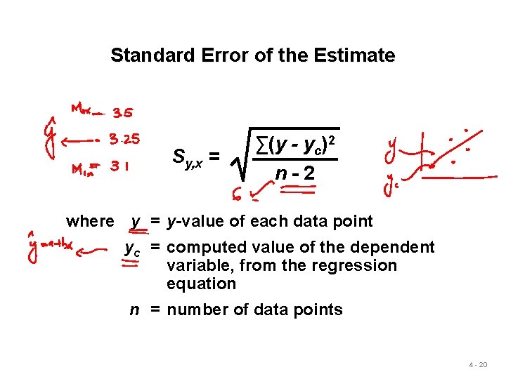
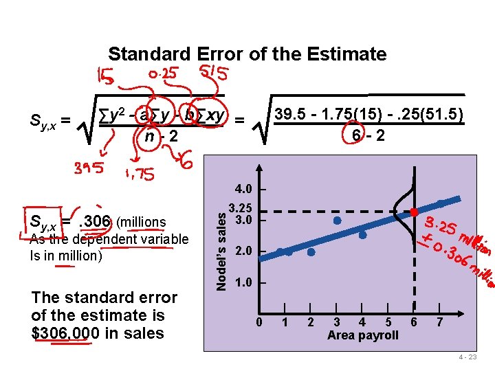
Standard Error of the Estimate Sy, x = ∑(y - yc)2 n-2 where y = y-value of each data point yc = computed value of the dependent variable, from the regression equation n = number of data points 4 - 20

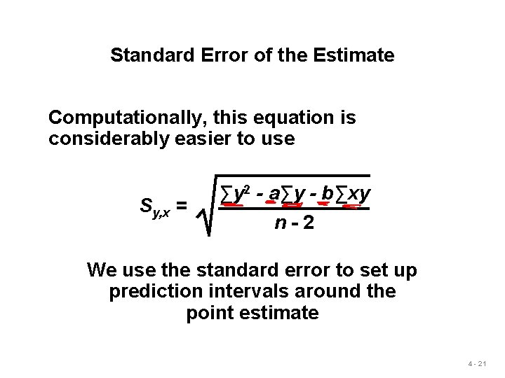
Standard Error of the Estimate Computationally, this equation is considerably easier to use Sy, x = ∑y 2 - a∑y - b∑xy n-2 We use the standard error to set up prediction intervals around the point estimate 4 - 21

Associative Forecasting Example Sales, y 2. 0 3. 0 2. 5 2. 0 3. 5 ∑y = 15. 0 Payroll, x 1 3 4 2 1 7 ∑x = 18 x = ∑x/6 = 18/6 = 3 y = ∑y/6 = 15/6 = 2. 5 b= x 2 1 9 16 4 1 49 ∑x 2 = 80 ∑xy - nxy ∑x 2 - nx 2 = xy 2. 0 9. 0 10. 0 4. 0 24. 5 ∑xy = 51. 5 - (6)(3)(2. 5) 80 - (6)(32) =. 25 a = y - bx = 2. 5 - (. 25)(3) = 1. 75 4 - 22

Standard Error of the Estimate Sy, x = 39. 5 - 1. 75(15) -. 25(51. 5) 6 -2 ∑y 2 - a∑y - b∑xy = n-2 Sy, x =. 306 (millions As the dependent variable Is in million) The standard error of the estimate is $306, 000 in sales Nodel’s sales 4. 0 – 3. 25 3. 0 – 2. 0 – 1. 0 – 0 | 1 | 2 | | 3 4 5 6 Area payroll | 7 4 - 23

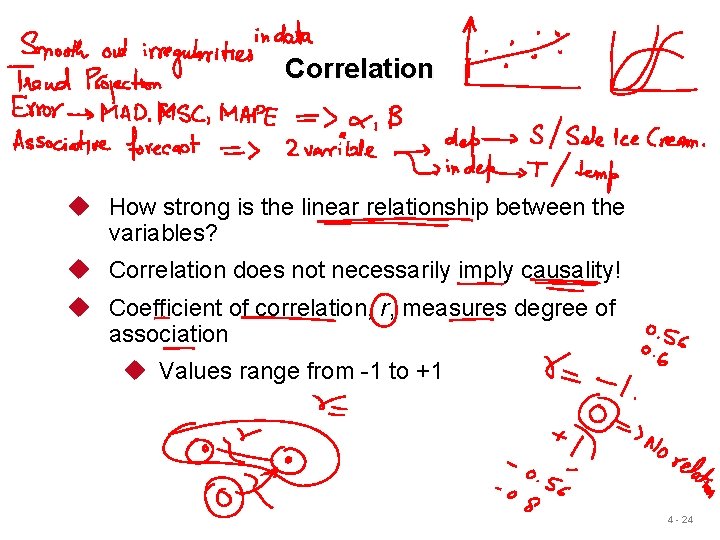
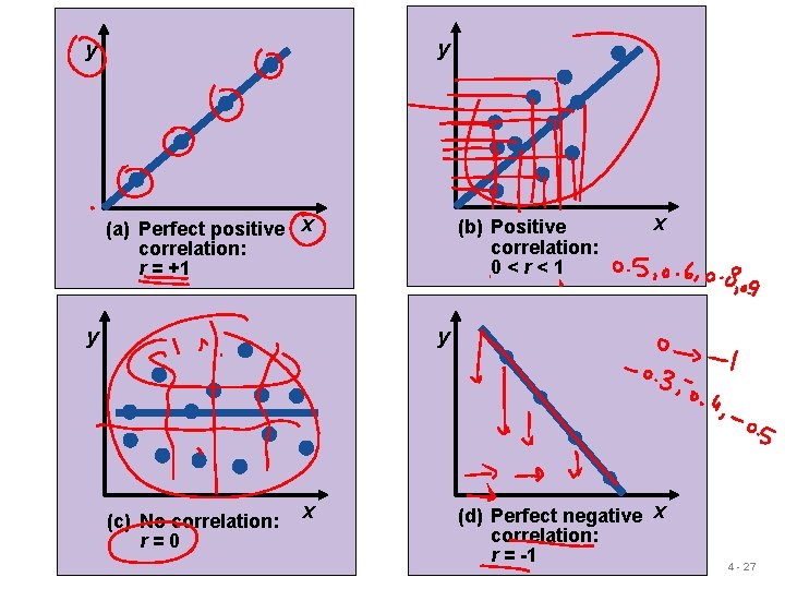
Correlation u How strong is the linear relationship between the variables? u Correlation does not necessarily imply causality! u Coefficient of correlation, r, measures degree of association u Values range from -1 to +1 4 - 24

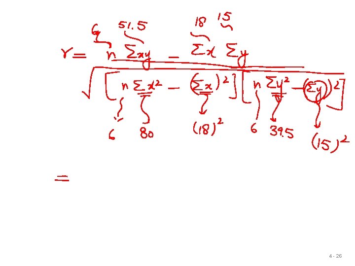
Correlation Coefficient r= n. Sxy - Sx. Sy [n. Sx 2 - (Sx)2][n. Sy 2 - (Sy)2] Sales, y 2. 0 3. 0 2. 5 2. 0 3. 5 ∑y = 15. 0 Payroll, x 1 3 4 2 1 7 ∑x = 18 x 2 1 9 16 4 1 49 ∑x 2 = 80 xy 2. 0 9. 0 10. 0 4. 0 24. 5 ∑xy = 51. 5 4 - 25

4 - 26

y y (a) Perfect positive x correlation: r = +1 y (b) Positive correlation: 0<r<1 x y (c) No correlation: r=0 x (d) Perfect negative x correlation: r = -1 4 - 27

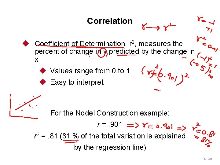
Correlation u Coefficient of Determination, r 2, measures the percent of change in y predicted by the change in x u Values range from 0 to 1 u Easy to interpret For the Nodel Construction example: r =. 901 r 2 =. 81 (81 % of the total variation is explained by the regression line) 4 - 28

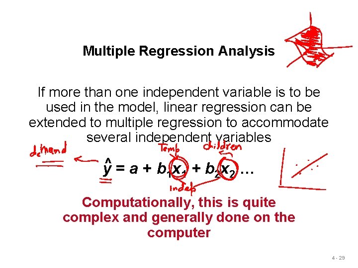
Multiple Regression Analysis If more than one independent variable is to be used in the model, linear regression can be extended to multiple regression to accommodate several independent variables y^ = a + b 1 x 1 + b 2 x 2 … Computationally, this is quite complex and generally done on the computer 4 - 29

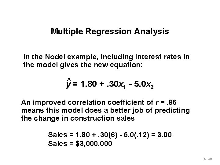
Multiple Regression Analysis In the Nodel example, including interest rates in the model gives the new equation: y^ = 1. 80 +. 30 x 1 - 5. 0 x 2 An improved correlation coefficient of r =. 96 means this model does a better job of predicting the change in construction sales Sales = 1. 80 +. 30(6) - 5. 0(. 12) = 3. 00 Sales = $3, 000 4 - 30

Summary of Today's Presentation u Time-Series Forecasting u Seasonal Variation in Data u Associative forecast u Standard error of estimate u Correlation u Multiple regression 4 - 31