Seasonal Adjustment and DEMETRA ESTP course EUROSTAT 3

Seasonal Adjustment and DEMETRA+ ESTP course EUROSTAT 3 – 5 May 2011 Dario Buono and Enrico Infante Unit B 2 – Research and Methodology © 2011 by EUROSTAT. All rights reserved. Open to the public 03/05/2011

Plan – May 3 th n n n n Brief review of Time Series Analysis Seasonality and its determinants Decomposition models Exploration tools Why Seasonal Adjustment? Step by step procedures for SA Using DEMETRA+ – Getting familiarity – First results 03/05/2011 ESTP course Dario Buono, Enrico Infante 2

Plan – May 4 th n Identification of type of outliers: – Additive Outlier – Transitory Change – Level Shift n Calendar Effect and its components n X-12 ARIMA vs Tramo/Seats n Using DEMETRA+ – Calendar Adjustment and outliers – Full exercise 03/05/2011 ESTP course Dario Buono, Enrico Infante 3

Plan – May 5 th n ESS Guidelines on SA: review n ESS Guidelines on SA: practical implementation n Using DEMETRA+ – Show and tell exercise by participants 03/05/2011 ESTP course Dario Buono, Enrico Infante 4

Session 1 – May 3 th Brief review of Time Series Analysis Seasonality and its determinants Decomposition models Exploration tools Why Seasonal Adjustment? Step by step procedures for SA 03/05/2011 ESTP course Dario Buono, Enrico Infante 5

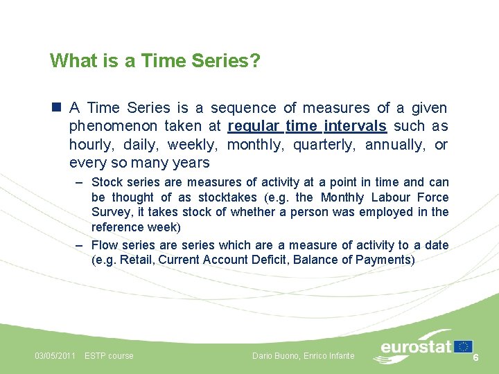
What is a Time Series? n A Time Series is a sequence of measures of a given phenomenon taken at regular time intervals such as hourly, daily, weekly, monthly, quarterly, annually, or every so many years – Stock series are measures of activity at a point in time and can be thought of as stocktakes (e. g. the Monthly Labour Force Survey, it takes stock of whether a person was employed in the reference week) – Flow series are series which are a measure of activity to a date (e. g. Retail, Current Account Deficit, Balance of Payments) 03/05/2011 ESTP course Dario Buono, Enrico Infante 6

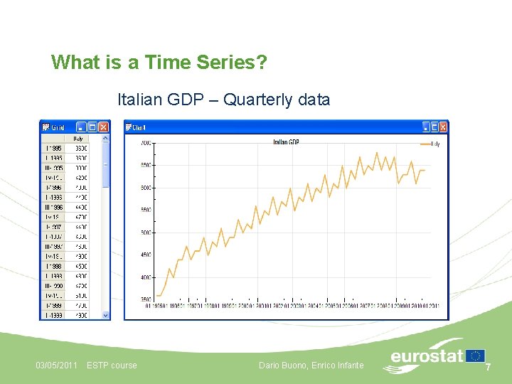
What is a Time Series? Italian GDP – Quarterly data 03/05/2011 ESTP course Dario Buono, Enrico Infante 7

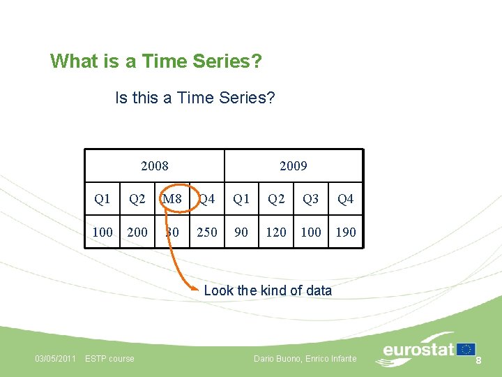
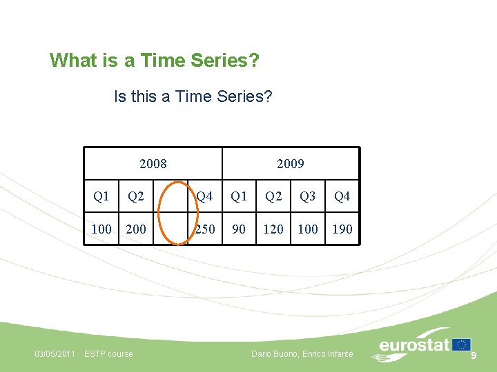
What is a Time Series? Is this a Time Series? 2008 Q 1 2009 Q 2 M 8 Q 4 Q 1 Q 2 Q 3 Q 4 100 200 30 250 90 120 100 190 Look the kind of data 03/05/2011 ESTP course Dario Buono, Enrico Infante 8

What is a Time Series? Is this a Time Series? 2008 Q 1 2009 Q 2 Q 4 Q 1 Q 2 100 250 90 120 100 190 03/05/2011 ESTP course Q 3 Q 4 Dario Buono, Enrico Infante 9

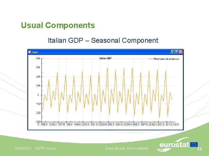
Usual Components n The Trend Component – The trend is the long-term evolution of the series that can be observed on several decades n The Cycle Component – The cycle is the smooth and quasi-periodic movement of the series that can usually be observed around the long term trend n The Seasonal Component (Seasonality) – Fluctuations observed during the year (each month, each quarter) and which appear to repeat themselves on a more or less regular basis from one year to other 03/05/2011 ESTP course Dario Buono, Enrico Infante 10

Usual Components n The Calendar Effect – Any economic effect which appears to be related to the calendar (one more Sunday in the month can affect the production) n The Irregular Component – The Irregular Component is composed of residual and random fluctuations that cannot be attributed to the other “systematic” components n Outliers 03/05/2011 ESTP course Dario Buono, Enrico Infante 11

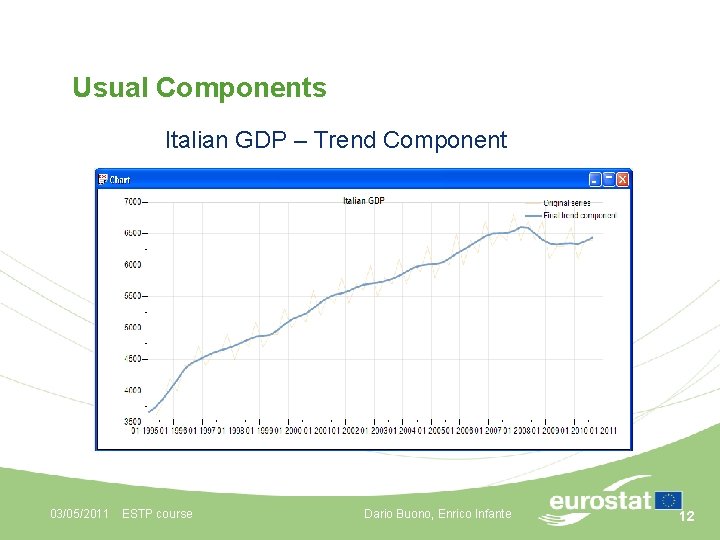
Usual Components Italian GDP – Trend Component 03/05/2011 ESTP course Dario Buono, Enrico Infante 12

Usual Components Italian GDP – Seasonal Component 03/05/2011 ESTP course Dario Buono, Enrico Infante 13

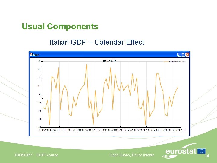
Usual Components Italian GDP – Calendar Effect 03/05/2011 ESTP course Dario Buono, Enrico Infante 14

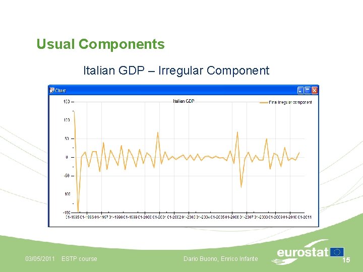
Usual Components Italian GDP – Irregular Component 03/05/2011 ESTP course Dario Buono, Enrico Infante 15

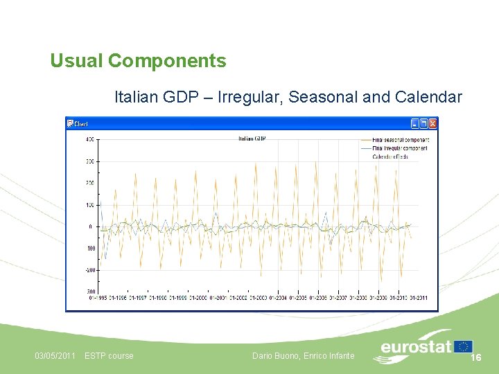
Usual Components Italian GDP – Irregular, Seasonal and Calendar 03/05/2011 ESTP course Dario Buono, Enrico Infante 16

Trend n The Trend Component is defined as the long term movement in a series n The trend is a reflection of the underlying level of the series. This is typically due to influences such as population growth, price inflation and general economic development n The Trend Component is sometimes referred to as the Trend-Cycle (see Cycle Component) 03/05/2011 ESTP course Dario Buono, Enrico Infante 17

Cause of Seasonality n Seasonality and Climate: due to the variations of the weather and of the climate (seasons!) – Examples: agriculture, consumption of electricity (heating) n Seasonality and Institutions: due to the social habits and practices or to the administrative rules – Examples: Effect of Christmas on the retail trade, of the fiscal year on some financial variables, of the academic calendar n Indirect Seasonality: due to the Seasonality that affects other sectors – Examples: toy industry is affected a long time before Christmas. A Seasonal increase in the retail trade has an impact on manufacturing, deliveries, etc. . 03/05/2011 ESTP course Dario Buono, Enrico Infante 18

Seasonal Adjustment n Seasonal Adjustment is the process of estimating and removing the Seasonal Effects from a Time Series, and by seasonal we mean an effect that happens at the same time and with the same magnitude and direction every year n The basic goal of Seasonal Adjustment is to decompose a Time Series into several different components including a Seasonal Component and an Irregular Component n Because the Seasonal effects are an unwanted feature of the Time Series, Seasonal Adjustment can be thought of as focused noise reduction 03/05/2011 ESTP course Dario Buono, Enrico Infante 19

Seasonal Adjustment n Since Seasonal effects are annual effects, the data must be collected at a frequency less than annually, usually monthly or quarterly n For the data to be useful for Time Series analysis, the data should be comparable over time. That means: – The measurements should be taken over discrete (nonoverlapping) consecutive periods, i. e. , every month or every quarter – The definition of the concept and the way it is measured should be consistent over time 03/05/2011 ESTP course Dario Buono, Enrico Infante 20

Seasonal Adjustment n Keep in mind that longer series aren't necessarily better. If the series has changed the way the data is measured or defined, it might be better to cut off the early part of the series to keep the series as homogeneous as possible n The best way to decide if your series needs to be shortened is to investigate the data collection methods and the economic factors associated with your series and choose a length that gives you the most homogeneous series possible 03/05/2011 ESTP course Dario Buono, Enrico Infante 21

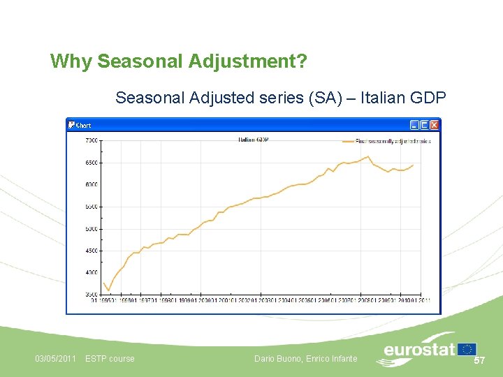
Seasonal Adjustment n During Seasonal Adjustment, we remove Seasonal effects from the original series. If present, we also remove Calendar Effects. The Seasonally Adjusted series is therefore a combination of the Trend and Irregular Components n One common misconception is that Seasonal Adjustment will also hide any outliers present. This is not the case: if there is some kind of unusual event, we need that information for analysis, and outliers are included in the Seasonally Adjusted series 03/05/2011 ESTP course Dario Buono, Enrico Infante 22

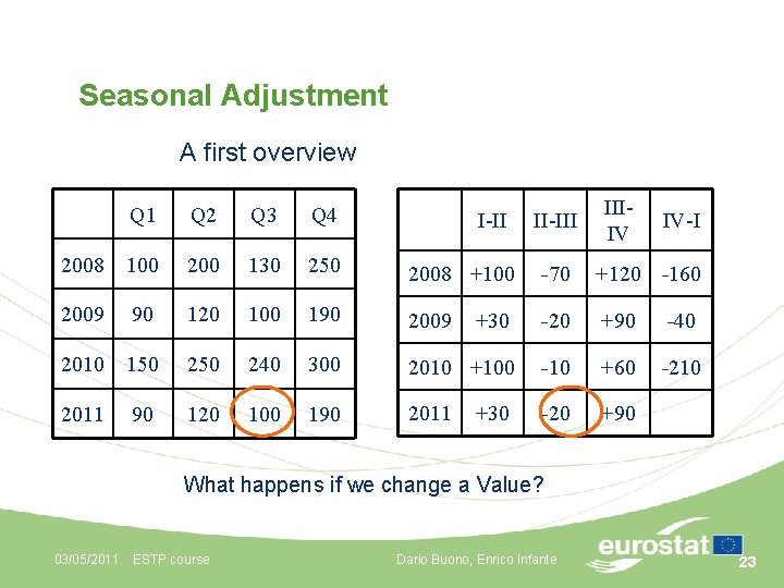
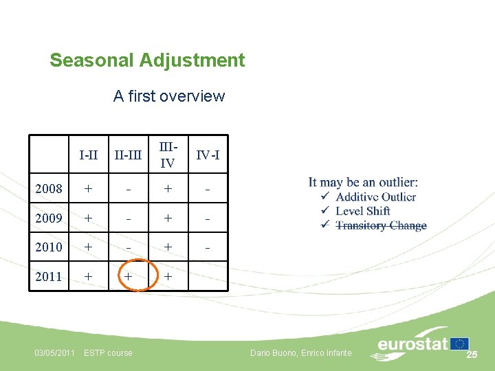
Seasonal Adjustment A first overview IIIIV Q 1 Q 2 Q 3 Q 4 2008 100 200 130 250 2008 +100 -70 +120 -160 2009 90 120 100 190 2009 +30 -20 +90 -40 2010 150 240 300 2010 +100 -10 +60 -210 2011 90 120 100 190 2011 -20 +90 I-II +30 II-III IV-I What happens if we change a Value? 03/05/2011 ESTP course Dario Buono, Enrico Infante 23

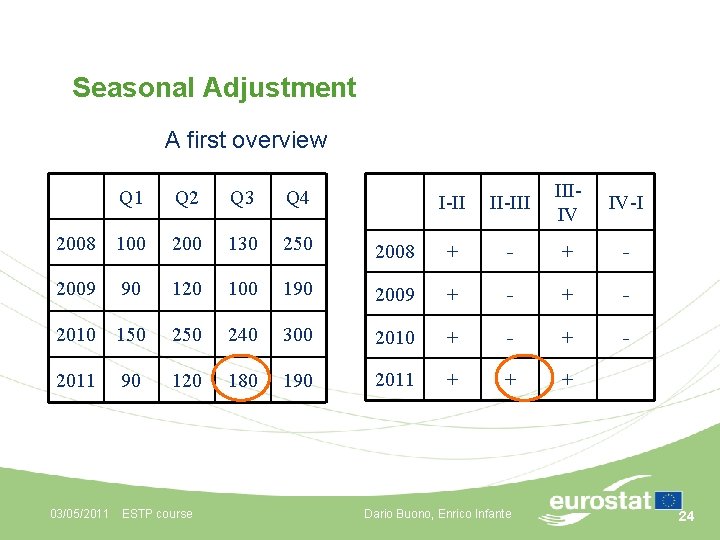
Seasonal Adjustment A first overview I-II II-III IIIIV IV-I 2008 + - 190 2009 + - 240 300 2010 + - 180 190 2011 + + + Q 1 Q 2 Q 3 Q 4 2008 100 200 130 250 2009 90 120 100 2010 150 2011 90 120 03/05/2011 ESTP course Dario Buono, Enrico Infante 24

Seasonal Adjustment A first overview I-II II-III IIIIV IV-I 2008 + - 2009 + - 2010 + - 2011 + + + 03/05/2011 ESTP course Dario Buono, Enrico Infante 25

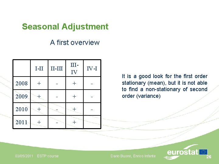
Seasonal Adjustment A first overview I-II II-III IIIIV IV-I 2008 + - 2009 + - 2010 + - 2011 + - + 03/05/2011 ESTP course It is a good look for the first order stationary (mean), but it is not able to find a non-stationary of second order (variance) Dario Buono, Enrico Infante 26

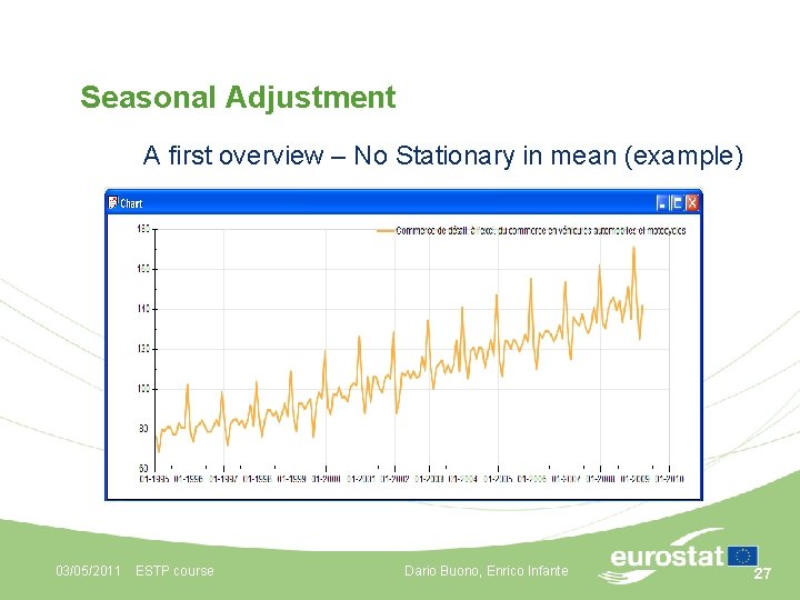
Seasonal Adjustment A first overview – No Stationary in mean (example) 03/05/2011 ESTP course Dario Buono, Enrico Infante 27

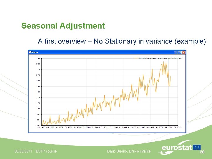
Seasonal Adjustment A first overview – No Stationary in variance (example) 03/05/2011 ESTP course Dario Buono, Enrico Infante 28

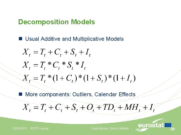
Decomposition Models n Usual Additive and Multiplicative Models n More components: Outliers, Calendar Effects 03/05/2011 ESTP course Dario Buono, Enrico Infante 29

Decomposition Models Some usual shapes 03/05/2011 ESTP course Dario Buono, Enrico Infante 30

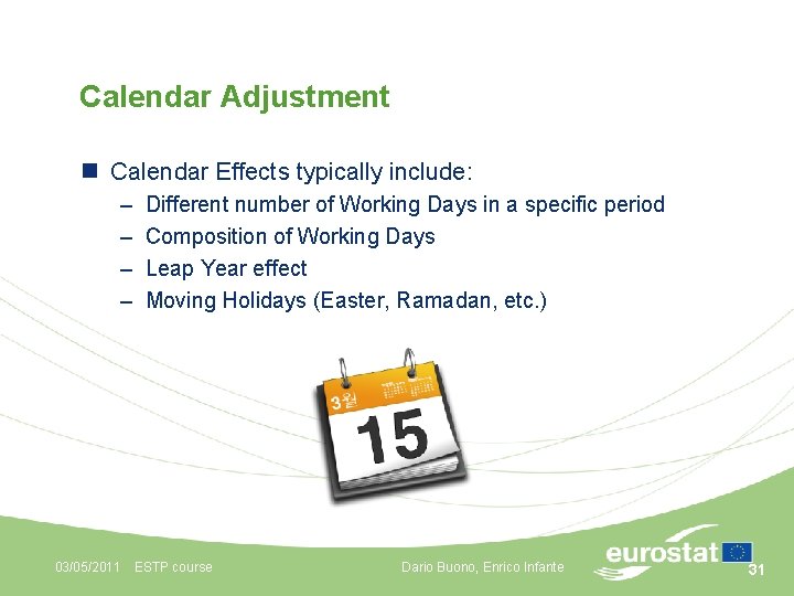
Calendar Adjustment n Calendar Effects typically include: – – Different number of Working Days in a specific period Composition of Working Days Leap Year effect Moving Holidays (Easter, Ramadan, etc. ) 03/05/2011 ESTP course Dario Buono, Enrico Infante 31

Calendar Adjustment – Trading Day Effect n Recurring effects associated with individual days of the week. This occurs because only non-leap-year Februaries have four of each type of day - four Mondays, four Tuesdays, etc. n All other months have an excess of some types of days. If an activity is higher on some days compared to others, then the series can have a Trading Day effect. For example, building permit offices are usually closed on Saturday and Sunday n Thus, the number of building permits issued in a given month is likely to be higher if the month contains a surplus of weekdays and lower if the month contains a surplus of weekend days 03/05/2011 ESTP course Dario Buono, Enrico Infante 32

Calendar Adjustment – Moving Holiday Effect n Effects from holidays that are not always on the same day of a month, such as Labor Day or Thanksgiving. The most important Moving Holiday in the US is Easter, not only because it moves between days, but can also move between months since it can occur in March or April 03/05/2011 ESTP course Dario Buono, Enrico Infante 33

Irregular Component n The Irregular Component is the remaining component of the series after the Seasonal and Trend Components have been removed from the original data n For this reason, it is also sometimes referred to as the Residual Component. It attempts to capture the remaining short term fluctuations in the series which are neither systematic nor predictable n The Irregular Component of a Time Series may or may not be random. It can contain both random effects (White Noise) or artifacts of non-sampling error, which are not necessarily random n Most Time Series contain some degree of volatility, causing original and Seasonally Adjusted values to oscillate around the general trend level. However, on occasions when the degree of irregularity is unusually large, the values can deviate from the Trend by a large margin, resulting in an extreme value. Some examples of the causes of extreme values are adverse natural events and industrial disputes 03/05/2011 ESTP course Dario Buono, Enrico Infante 34

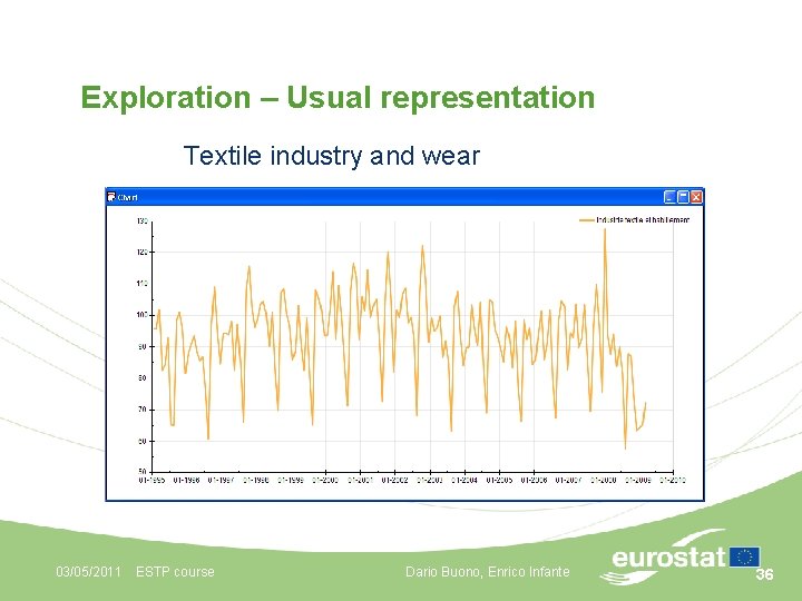
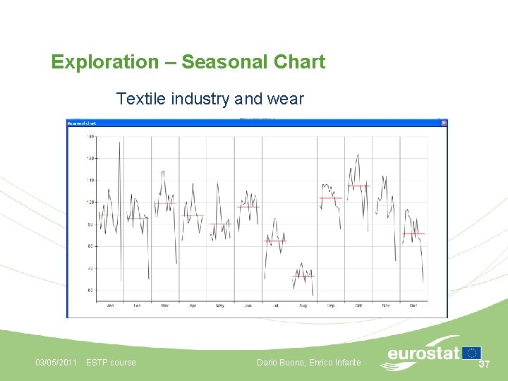
Exploration – Basic tools n Exploration is a very essential step when analyzing a Time Series n Looking for “structures” in the series – Trend, Seasonality, “strange” points or behavior etc. n Helps to formulate a global or decomposition model for the series n Graphics are a key player in this exploration 03/05/2011 ESTP course Dario Buono, Enrico Infante 35

Exploration – Usual representation Textile industry and wear 03/05/2011 ESTP course Dario Buono, Enrico Infante 36

Exploration – Seasonal Chart Textile industry and wear 03/05/2011 ESTP course Dario Buono, Enrico Infante 37

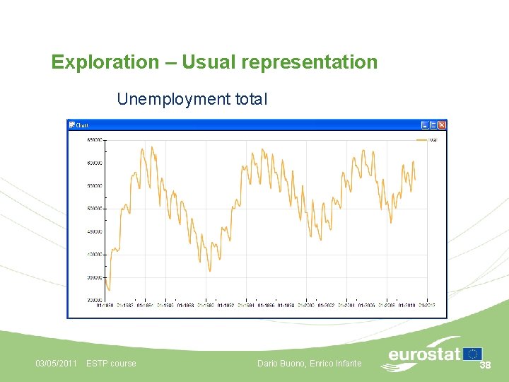
Exploration – Usual representation Unemployment total 03/05/2011 ESTP course Dario Buono, Enrico Infante 38

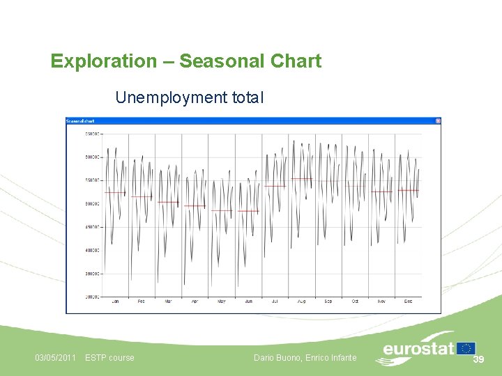
Exploration – Seasonal Chart Unemployment total 03/05/2011 ESTP course Dario Buono, Enrico Infante 39

Coffee-Break!!! We will restart in 15 minutes 03/05/2011 ESTP course Dario Buono, Enrico Infante 40

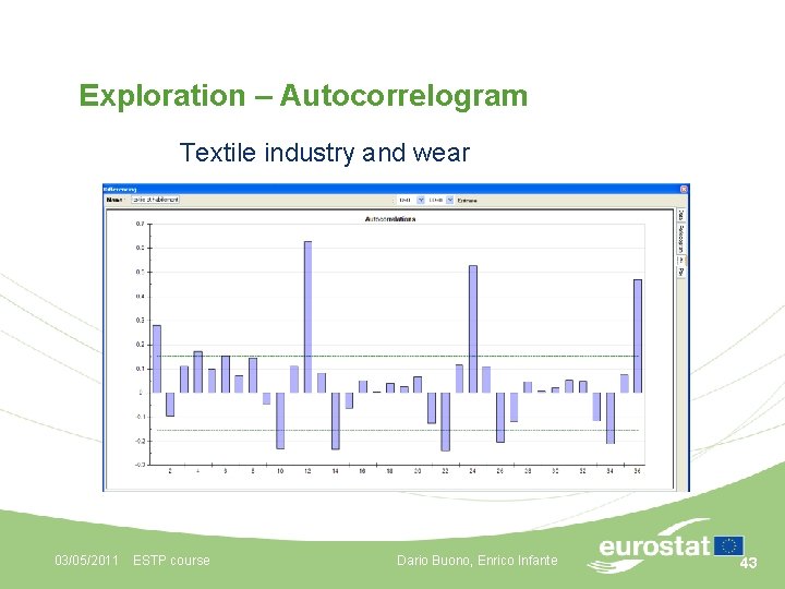
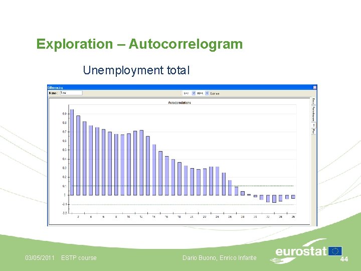
Exploration – Advanced tools n Two very important and useful graphics n Autocorrelogram – Shows the correlations between the series and itself (lagged series: 1, 2, 3… period lag) – See ARIMA modeling n Spectrum – Shows the frequencies that compose the series (as for a light or a sound) – Based on J. B. Fourier’s works (1807) 03/05/2011 ESTP course Dario Buono, Enrico Infante 41

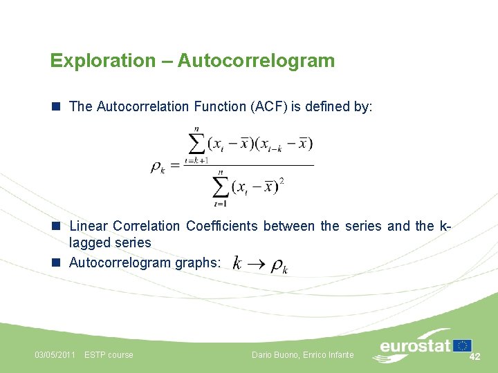
Exploration – Autocorrelogram n The Autocorrelation Function (ACF) is defined by: n Linear Correlation Coefficients between the series and the klagged series n Autocorrelogram graphs: 03/05/2011 ESTP course Dario Buono, Enrico Infante 42

Exploration – Autocorrelogram Textile industry and wear 03/05/2011 ESTP course Dario Buono, Enrico Infante 43

Exploration – Autocorrelogram Unemployment total 03/05/2011 ESTP course Dario Buono, Enrico Infante 44

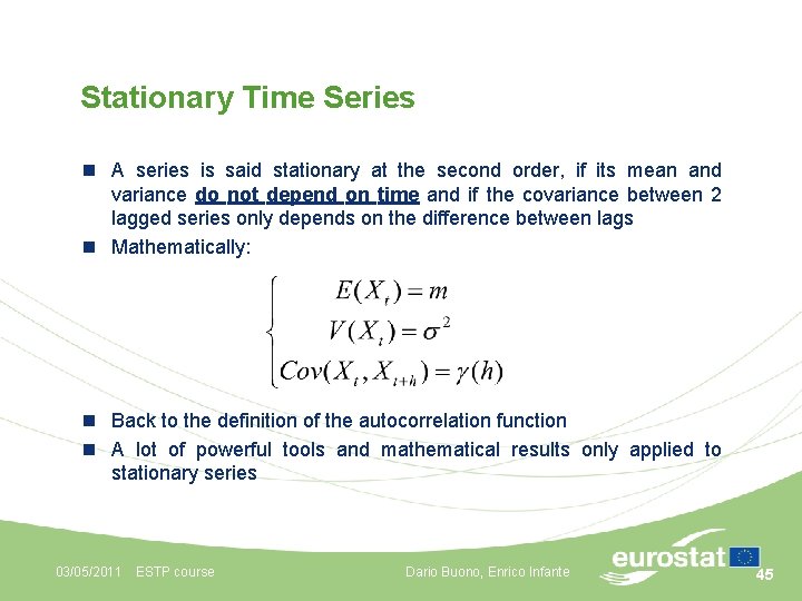
Stationary Time Series n A series is said stationary at the second order, if its mean and variance do not depend on time and if the covariance between 2 lagged series only depends on the difference between lags n Mathematically: n Back to the definition of the autocorrelation function n A lot of powerful tools and mathematical results only applied to stationary series 03/05/2011 ESTP course Dario Buono, Enrico Infante 45

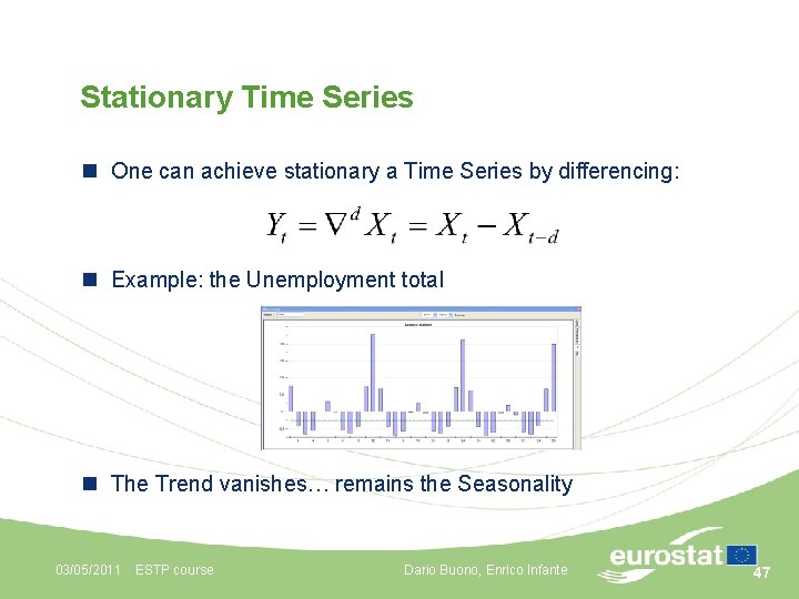
Stationary Time Series n One can achieve stationary a Time Series by differencing: n Example: the Unemployment total n The Trend vanishes… remains the Seasonality 03/05/2011 ESTP course Dario Buono, Enrico Infante 47

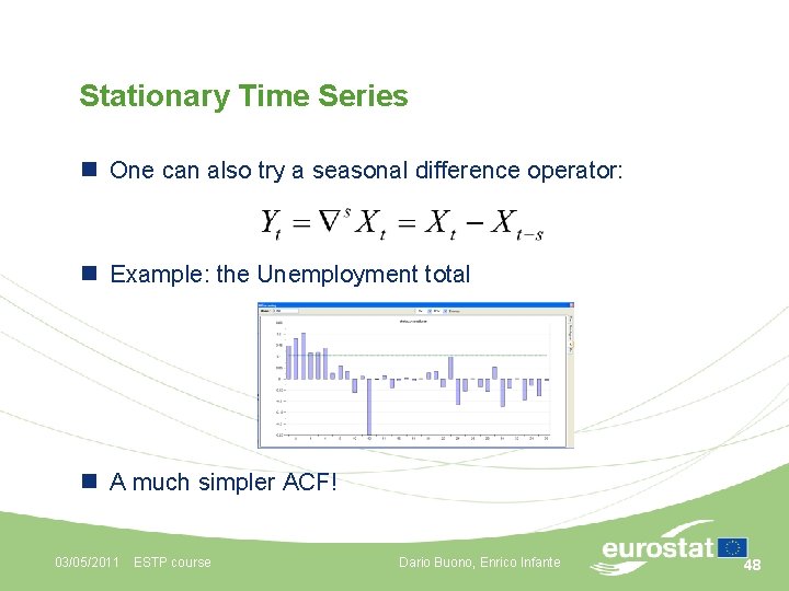
Stationary Time Series n One can also try a seasonal difference operator: n Example: the Unemployment total n A much simpler ACF! 03/05/2011 ESTP course Dario Buono, Enrico Infante 48

Stationary Time Series Some usual shapes 03/05/2011 ESTP course Dario Buono, Enrico Infante 49

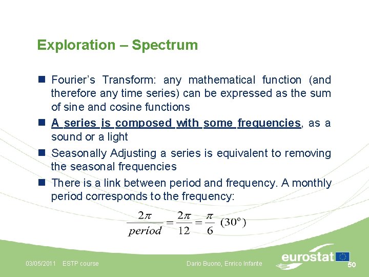
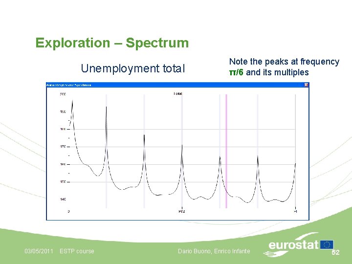
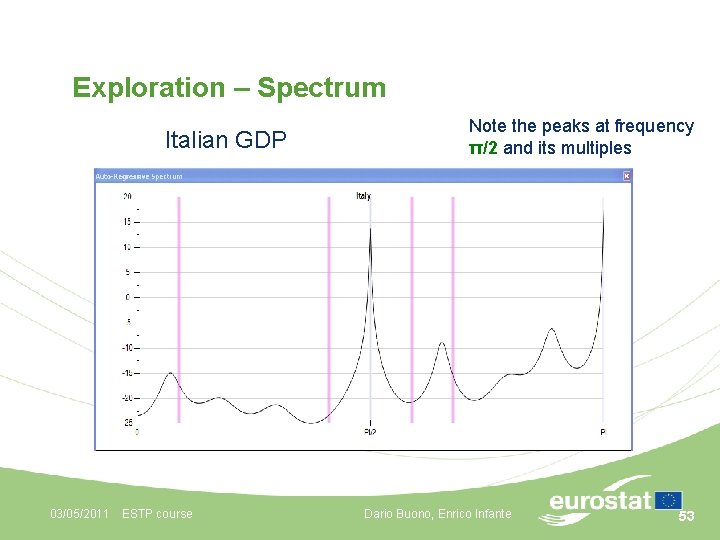
Exploration – Spectrum n Fourier’s Transform: any mathematical function (and therefore any time series) can be expressed as the sum of sine and cosine functions n A series is composed with some frequencies, as a sound or a light n Seasonally Adjusting a series is equivalent to removing the seasonal frequencies n There is a link between period and frequency. A monthly period corresponds to the frequency: 03/05/2011 ESTP course Dario Buono, Enrico Infante 50

Exploration – Spectrum n The spectrum is the graph which associates to a frequency its importance in the series n Important frequencies are therefore associated to a spectral peak n The estimation of the spectrum is a complex operation and, in theory, a spectrum is only defined for a stationary Time Series 03/05/2011 ESTP course Dario Buono, Enrico Infante 51

Exploration – Spectrum Unemployment total 03/05/2011 ESTP course Note the peaks at frequency π/6 and its multiples Dario Buono, Enrico Infante 52

Exploration – Spectrum Italian GDP 03/05/2011 ESTP course Note the peaks at frequency π/2 and its multiples Dario Buono, Enrico Infante 53

Exploration – Spectrum Some usual shapes 03/05/2011 ESTP course Dario Buono, Enrico Infante 54

Why Seasonal Adjustment? n Business cycle analysis n To improve comparability: – Over time: • Example: how to compare the first quarter (with February) to the fourth quarter (with Christmas)? – Across space: • Never forget that when we are freezing at work, Australians are burning on the beach! • Very important to compare European national economies (convergence of business cycles) or sectors 03/05/2011 ESTP course Dario Buono, Enrico Infante 55

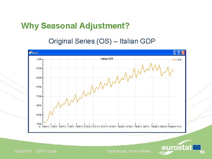
Why Seasonal Adjustment? Original Series (OS) – Italian GDP 03/05/2011 ESTP course Dario Buono, Enrico Infante 56

Why Seasonal Adjustment? Seasonal Adjusted series (SA) – Italian GDP 03/05/2011 ESTP course Dario Buono, Enrico Infante 57

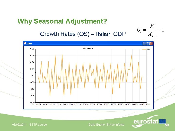
Why Seasonal Adjustment? Growth Rates (OS) – Italian GDP 03/05/2011 ESTP course Dario Buono, Enrico Infante 58

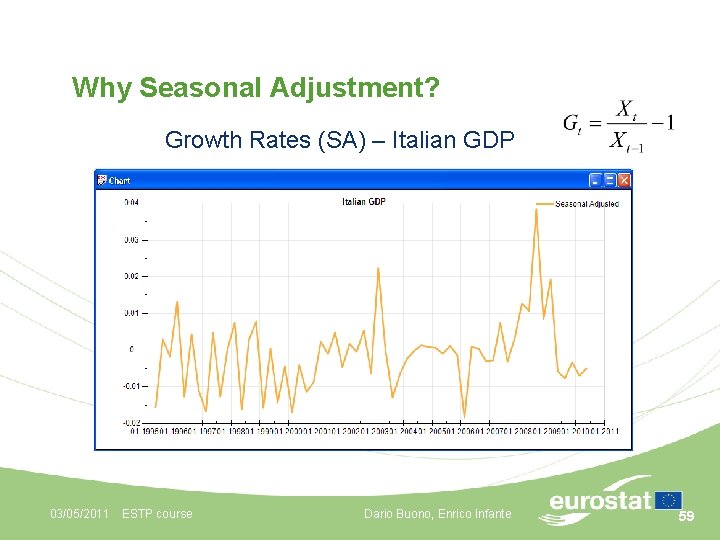
Why Seasonal Adjustment? Growth Rates (SA) – Italian GDP 03/05/2011 ESTP course Dario Buono, Enrico Infante 59

Why Seasonal Adjustment? n The aim of Seasonal Adjustment is to eliminate Seasonal and Calendar Effects. Hence there are no Seasonal and Calendar Effects in a perfectly Seasonally Adjusted series n In other words: Seasonal Adjustment transforms the world we live in into a world where no Seasonal and Calendar Effects occur. In a Seasonally Adjusted world the temperature is exactly the same in winter as in the summer, there are no holidays, Christmas is abolished, people work every day in the week with the same intensity (no break over the weekend), etc. 03/05/2011 ESTP course Dario Buono, Enrico Infante 60

Step by step procedures for SA n Step 0: Number of observations – It is a requirement for Seasonal Adjustment that the Times Series have to be at least 3 years-long (36 observations) for monthly series and 4 years-long (16 observations) for quarterly series. If a series does not fulfill this condition, it is not long enough for Seasonal Adjustment. Of course these are minimum values, series can be longer for an adequate adjustment or for the computation of diagnostics depending on the fitted ARIMA model 03/05/2011 ESTP course Dario Buono, Enrico Infante 61

Step by step procedures for SA n Step 1: Graph – It is important to have a look at the data and graph of the original Time Series before running a Seasonal Adjustment method – Series with possible outlier values should be identified. Verification is needed concerning that the outliers are valid and there is not sign problem in the data for example captured erroneously – The missing observations in the Time Series should be identified and explained. Series with too many missing values will cause estimation problems – If series are part of an aggregate series, it should be verified that the starting and ending dates for all component series are the same – Look at the Spectral Graph of the Original Series (optional) 03/05/2011 ESTP course Dario Buono, Enrico Infante 62

Step by step procedures for SA n Step 2: Constant in variance – – – The type of transformation should be used automatically. Confirm the results of the automatic choice by looking at graphs of the series. If the diagnostics for choosing between additive and multiplicative adjustments are inconclusive, then you can chose to continue with the type of transformation used in the past to allow for consistency between years or it is recommended to visually inspect the graph of the series If the series has zero and negative values, then this series must be additively adjusted If the series has a decreasing level with positive values close to zero, then multiplicative adjustment must be used 03/05/2011 ESTP course Dario Buono, Enrico Infante 63

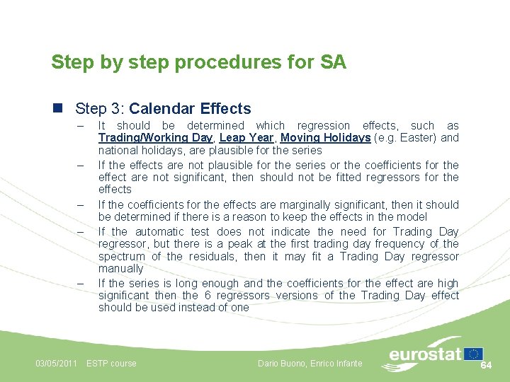
Step by step procedures for SA n Step 3: Calendar Effects – – – It should be determined which regression effects, such as Trading/Working Day, Leap Year, Moving Holidays (e. g. Easter) and national holidays, are plausible for the series If the effects are not plausible for the series or the coefficients for the effect are not significant, then should not be fitted regressors for the effects If the coefficients for the effects are marginally significant, then it should be determined if there is a reason to keep the effects in the model If the automatic test does not indicate the need for Trading Day regressor, but there is a peak at the first trading day frequency of the spectrum of the residuals, then it may fit a Trading Day regressor manually If the series is long enough and the coefficients for the effect are high significant then the 6 regressors versions of the Trading Day effect should be used instead of one 03/05/2011 ESTP course Dario Buono, Enrico Infante 64

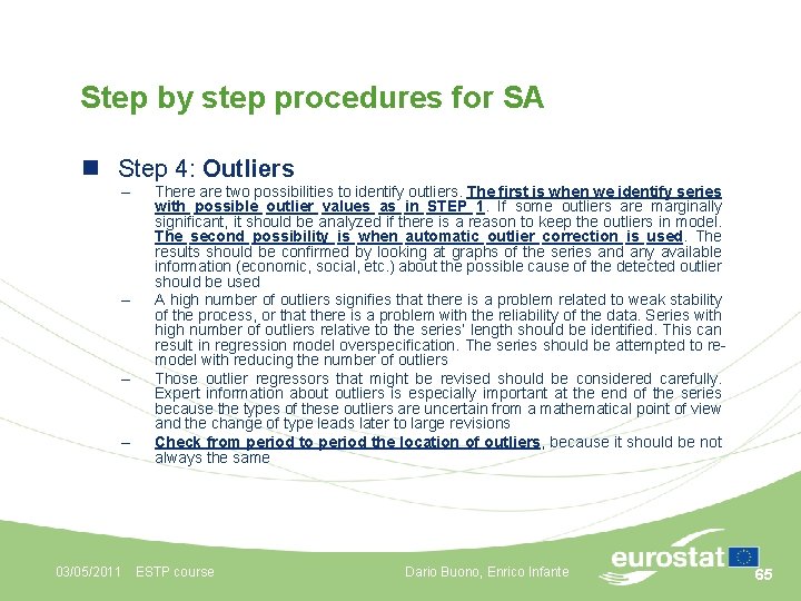
Step by step procedures for SA n Step 4: Outliers – – There are two possibilities to identify outliers. The first is when we identify series with possible outlier values as in STEP 1. If some outliers are marginally significant, it should be analyzed if there is a reason to keep the outliers in model. The second possibility is when automatic outlier correction is used. The results should be confirmed by looking at graphs of the series and any available information (economic, social, etc. ) about the possible cause of the detected outlier should be used A high number of outliers signifies that there is a problem related to weak stability of the process, or that there is a problem with the reliability of the data. Series with high number of outliers relative to the series’ length should be identified. This can result in regression model overspecification. The series should be attempted to remodel with reducing the number of outliers Those outlier regressors that might be revised should be considered carefully. Expert information about outliers is especially important at the end of the series because the types of these outliers are uncertain from a mathematical point of view and the change of type leads later to large revisions Check from period to period the location of outliers, because it should be not always the same 03/05/2011 ESTP course Dario Buono, Enrico Infante 65

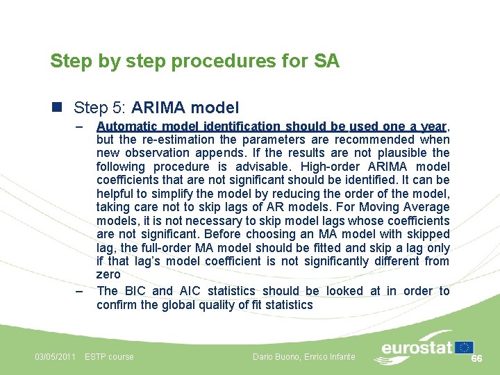
Step by step procedures for SA n Step 5: ARIMA model – – Automatic model identification should be used one a year, but the re-estimation the parameters are recommended when new observation appends. If the results are not plausible the following procedure is advisable. High-order ARIMA model coefficients that are not significant should be identified. It can be helpful to simplify the model by reducing the order of the model, taking care not to skip lags of AR models. For Moving Average models, it is not necessary to skip model lags whose coefficients are not significant. Before choosing an MA model with skipped lag, the full-order MA model should be fitted and skip a lag only if that lag’s model coefficient is not significantly different from zero The BIC and AIC statistics should be looked at in order to confirm the global quality of fit statistics 03/05/2011 ESTP course Dario Buono, Enrico Infante 66

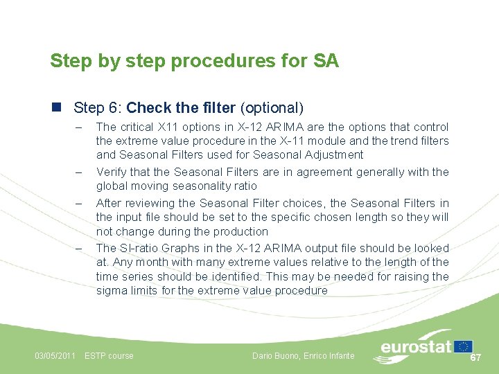
Step by step procedures for SA n Step 6: Check the filter (optional) – – The critical X 11 options in X-12 ARIMA are the options that control the extreme value procedure in the X-11 module and the trend filters and Seasonal Filters used for Seasonal Adjustment Verify that the Seasonal Filters are in agreement generally with the global moving seasonality ratio After reviewing the Seasonal Filter choices, the Seasonal Filters in the input file should be set to the specific chosen length so they will not change during the production The SI-ratio Graphs in the X-12 ARIMA output file should be looked at. Any month with many extreme values relative to the length of the time series should be identified. This may be needed for raising the sigma limits for the extreme value procedure 03/05/2011 ESTP course Dario Buono, Enrico Infante 67

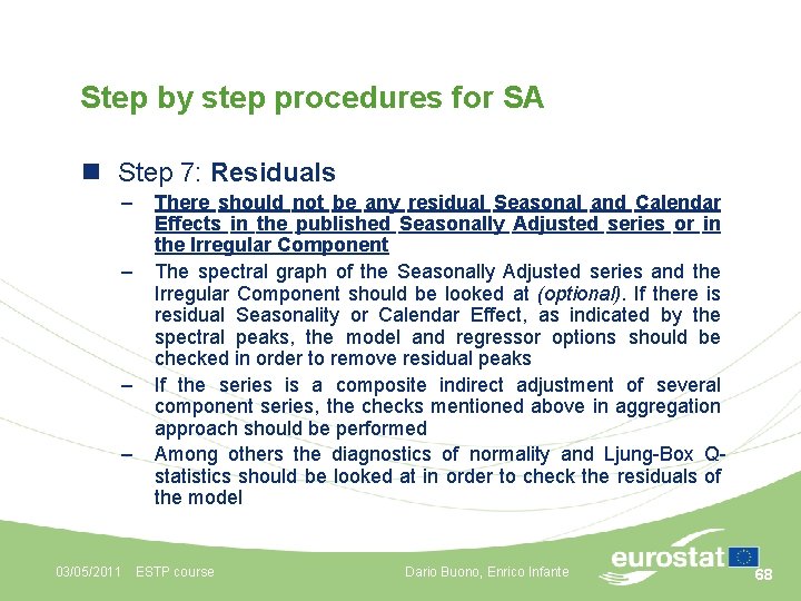
Step by step procedures for SA n Step 7: Residuals – – There should not be any residual Seasonal and Calendar Effects in the published Seasonally Adjusted series or in the Irregular Component The spectral graph of the Seasonally Adjusted series and the Irregular Component should be looked at (optional). If there is residual Seasonality or Calendar Effect, as indicated by the spectral peaks, the model and regressor options should be checked in order to remove residual peaks If the series is a composite indirect adjustment of several component series, the checks mentioned above in aggregation approach should be performed Among others the diagnostics of normality and Ljung-Box Qstatistics should be looked at in order to check the residuals of the model 03/05/2011 ESTP course Dario Buono, Enrico Infante 68

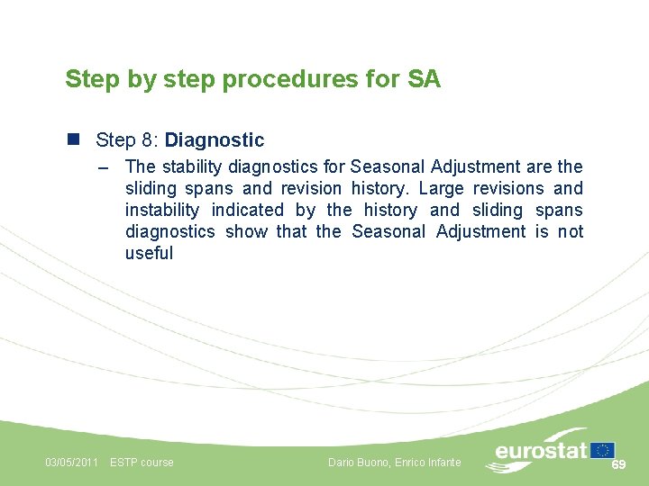
Step by step procedures for SA n Step 8: Diagnostic – The stability diagnostics for Seasonal Adjustment are the sliding spans and revision history. Large revisions and instability indicated by the history and sliding spans diagnostics show that the Seasonal Adjustment is not useful 03/05/2011 ESTP course Dario Buono, Enrico Infante 69

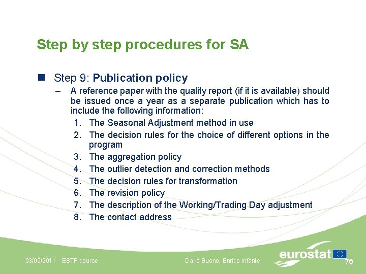
Step by step procedures for SA n Step 9: Publication policy – A reference paper with the quality report (if it is available) should be issued once a year as a separate publication which has to include the following information: 1. The Seasonal Adjustment method in use 2. The decision rules for the choice of different options in the program 3. The aggregation policy 4. The outlier detection and correction methods 5. The decision rules for transformation 6. The revision policy 7. The description of the Working/Trading Day adjustment 8. The contact address 03/05/2011 ESTP course Dario Buono, Enrico Infante 70

Questions? 03/05/2011 ESTP course Dario Buono, Enrico Infante 71