Introduction to Parallel Programming Message Passing Francisco Almeida

Introduction to Parallel Programming (Message Passing) Francisco Almeida falmeida@ull. es Parallel Computing Group

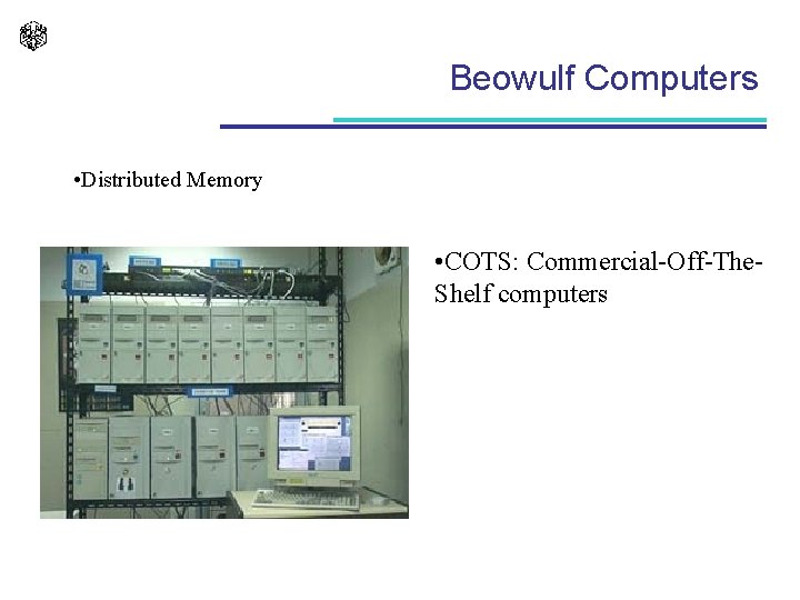
Beowulf Computers • Distributed Memory • COTS: Commercial-Off-The. Shelf computers

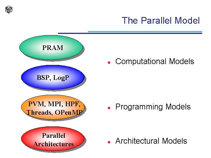
The Parallel Model PRAM l Computational Models l Programming Models l Architectural Models BSP, Log. P PVM, MPI, HPF, Threads, OPen. MP Parallel Architectures

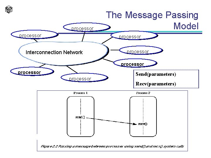
processor The Message Passing Model processor Interconnection Network processor Send(parameters) Recv(parameters)

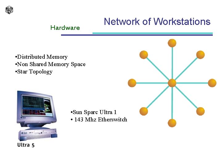
Hardware Network of Workstations • Distributed Memory • Non Shared Memory Space • Star Topology • Sun Sparc Ultra 1 • 143 Mhz Etherswitch

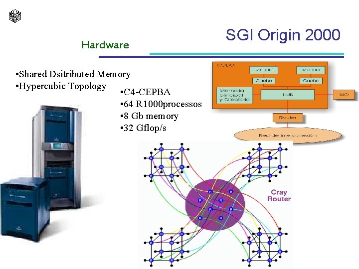
Hardware • Shared Dsitributed Memory • Hypercubic Topology • C 4 -CEPBA • 64 R 1000 processos • 8 Gb memory • 32 Gflop/s SGI Origin 2000

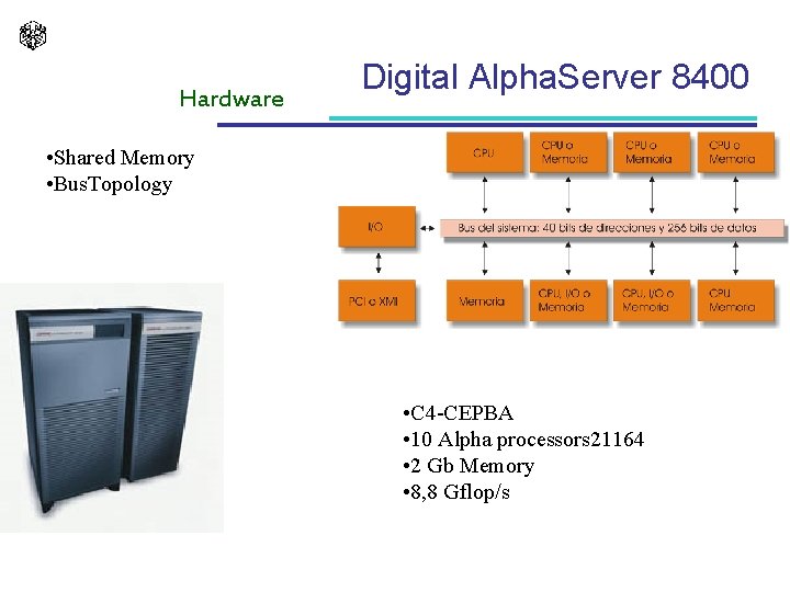
Hardware Digital Alpha. Server 8400 • Shared Memory • Bus. Topology • C 4 -CEPBA • 10 Alpha processors 21164 • 2 Gb Memory • 8, 8 Gflop/s

Drawbacks that arise when solving Problems using Parallelism l l l Parallel Programming is more complex than sequential. Results may vary as a consequence of the intrinsic non determinism. New problems. Deadlocks, starvation. . . Is more difficult to debug parallel programs. Parallel programs are less portable.

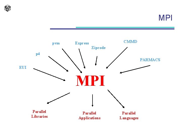
MPI pvm CMMD Express Zipcode p 4 PARMACS EUI MPI Parallel Libraries Parallel Applications Parallel Languages

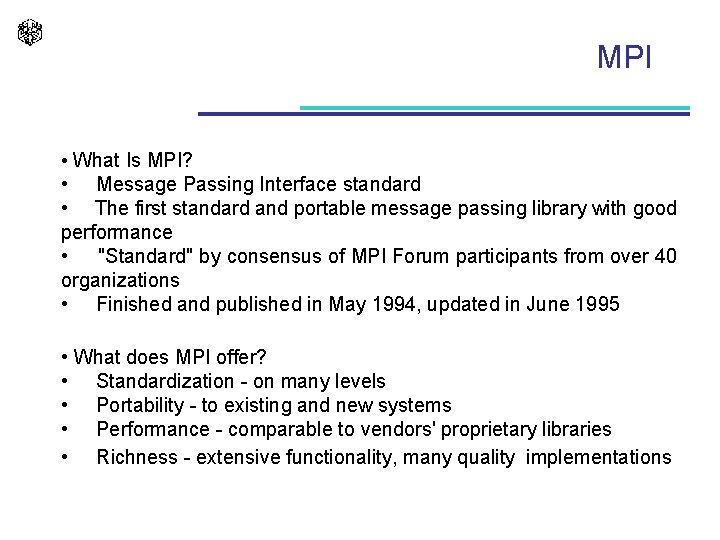
MPI • What Is MPI? • Message Passing Interface standard • The first standard and portable message passing library with good performance • "Standard" by consensus of MPI Forum participants from over 40 organizations • Finished and published in May 1994, updated in June 1995 • What does MPI offer? • Standardization - on many levels • Portability - to existing and new systems • Performance - comparable to vendors' proprietary libraries • Richness - extensive functionality, many quality implementations

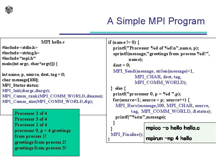
A Simple MPI Program MPI hello. c #include <stdio. h> #include <string. h> #include "mpi. h" main(int argc, char*argv[]) { int name, p, source, dest, tag = 0; char message[100]; MPI_Status status; MPI_Init(&argc, &argv); MPI_Comm_rank(MPI_COMM_WORLD, &name); MPI_Comm_size(MPI_COMM_WORLD, &p); Processor 2 of 4 Processor 3 of 4 Processor 1 of 4 processor 0, p = 4 greetings from process 1! greetings from process 2! greetings from process 3! if (name != 0) { printf("Processor %d of %dn", name, p); sprintf(message, "greetings from process %d!", name); dest = 0; MPI_Send(message, strlen(message)+1, MPI_CHAR, dest, tag, MPI_COMM_WORLD); } else { printf("processor 0, p = %d ", p); for(source=1; source < p; source++) { MPI_Recv(message, 100, MPI_CHAR, source, tag, MPI_COMM_WORLD, &status); printf("%sn", message); } mpicc –o hello. c } MPI_Finalize(); } mpirun –np 4 hello

Basic Communication Operations

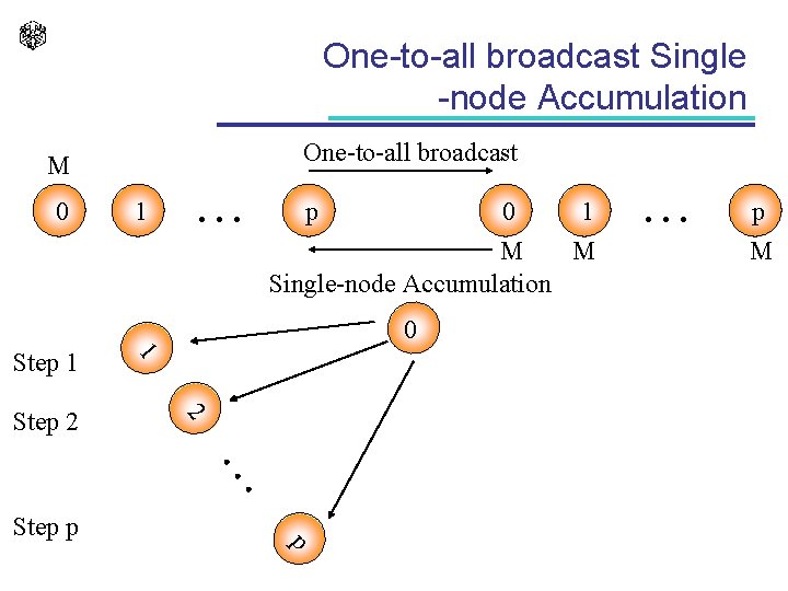
One-to-all broadcast Single -node Accumulation One-to-all broadcast M 0 1 . . . p 0 1 M M Single-node Accumulation 0 2 Step 2 1 Step 1 . . . Step p . . . p M p

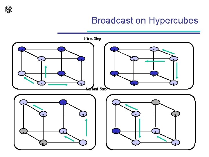
Broadcast on Hypercubes First Step 6 7 2 4 6 3 2 5 0 6 4 1 7 2 4 0 Second Step 3 1 7 2 4 1 3 5 6 5 0 7 3 5 0 1

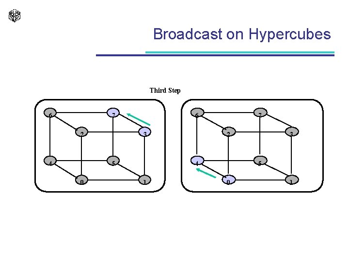
Broadcast on Hypercubes Third Step 6 7 2 4 6 3 5 0 7 2 4 1 3 5 0 1

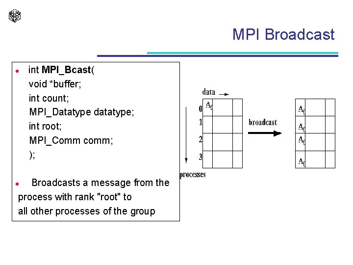
MPI Broadcast l int MPI_Bcast( void *buffer; int count; MPI_Datatype datatype; int root; MPI_Comm comm; ); Broadcasts a message from the process with rank "root" to all other processes of the group l

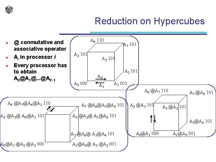
Reduction on Hypercubes l l l @ conmutative and associative operator Ai in processor i Every processor has to obtain A 0@A 1@. . . @AP-1 A 6 @A 7@A 4@A 5 110 A 2 @A 3@ A 0@A 1 101 A 6 110 A 2 101 A 7 101 A 3 101 A 5 101 A 0 000 A 1 001 A 7 @A 6@A 5@A 4 101 A 2 @A 3 101 A 3 @A 2@ A 1@A 0 101 A 7 @A 6@ A 5@A 4 101 A 0@A 1 @A 2 @A 3 000 A 6 @A 7 110 A 1@A 0@ A 3 @A 2 001 A 7 @A 6 101 A 3 @A 2 101 A 5@A 4 101 A 0@A 1 000 A 1@A 0 001

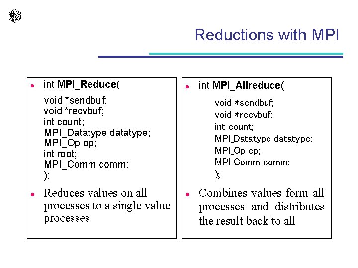
Reductions with MPI l int MPI_Reduce( l void *sendbuf; void *recvbuf; int count; MPI_Datatype datatype; MPI_Op op; int root; MPI_Comm comm; ); l Reduces values on all processes to a single value processes int MPI_Allreduce( void *sendbuf; void *recvbuf; int count; MPI_Datatype datatype; MPI_Op op; MPI_Comm comm; ); l Combines values form all processes and distributes the result back to all

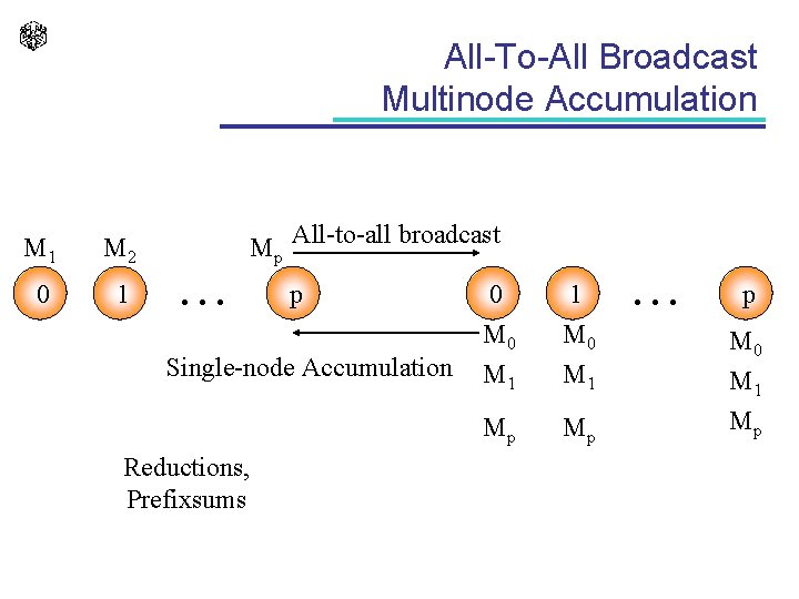
All-To-All Broadcast Multinode Accumulation M 1 M 2 0 1 Mp All-to-all broadcast . . . p Single-node Accumulation Reductions, Prefixsums 0 M 1 1 M 0 M 1 Mp Mp . . . p M 0 M 1 Mp

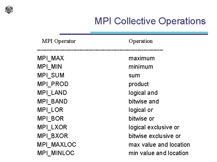
MPI Collective Operations MPI Operator Operation -------------------------------MPI_MAX maximum MPI_MIN minimum MPI_SUM sum MPI_PROD product MPI_LAND logical and MPI_BAND bitwise and MPI_LOR logical or MPI_BOR bitwise or MPI_LXOR logical exclusive or MPI_BXOR bitwise exclusive or MPI_MAXLOC max value and location MPI_MINLOC min value and location

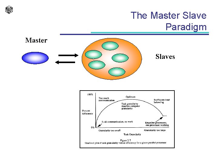
The Master Slave Paradigm Master Slaves

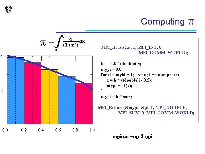
Computing 1 = 4 dx (1+x 2) MPI_Bcast(&n, 1, MPI_INT, 0, MPI_COMM_WORLD); 0 4 h = 1. 0 / (double) n; mypi = 0. 0; for (i = myid + 1; i <= n; i += numprocs) { x = h * ((double)i - 0. 5); mypi += f(x); } mypi = h * sum; 2 MPI_Reduce(&mypi, &pi, 1, MPI_DOUBLE, MPI_SUM, 0, MPI_COMM_WORLD); 0. 0 0. 2 0. 4 0. 6 0. 8 1. 0 mpirun –np 3 cpi

The Portability of the Efficiency

The Sequential Algorithm f[k][c] = max {f[k-1][C], f[k-1][C - W[k] ] + p[k ] for C W[k]} . . . n. . void mochila 01_sec (void) { unsigned v 1; int c, k; for (c = 0; c <= C; c++) f[0][c] = 0; for (k = 1; k <= N; k++) { for (c = 0; c <= C; c++) f[k][c] = f[k-1][c]; if (c >= w[k]) v 1 = f[k-1][c w[k]] + p[k]; if (f[k][c] > v 1) f[k][c] = v 1; } C. . l f[k -] 1] f[k] O(n*C)

The Parallel Algorithm . . . . Processor k f[k-1][c] . . . . c. . 8: for (c = 0; c <= C; c++) { 9: IN(&x); 10: f[c] = max(f[c], x); 11: OUT(&f[c], 1, sizeof(unsigned)); 12: if (C >= c + w[k]) 13: f[c + w[k]] = x + p[k]; 14: } 15: } Processor k - 1 . . 1: void transition (int stage) 2: { 3: unsigned x; 4: int c, k; 5: k = stage; 6: for (c = 0; c <= C; c++) 7: f[c] = 0; f[k][c] = max {f[k-1][C], f[k-1][C - W[k] ] + p[k]}

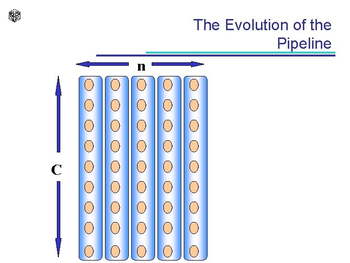
The Evolution of the Pipeline n C

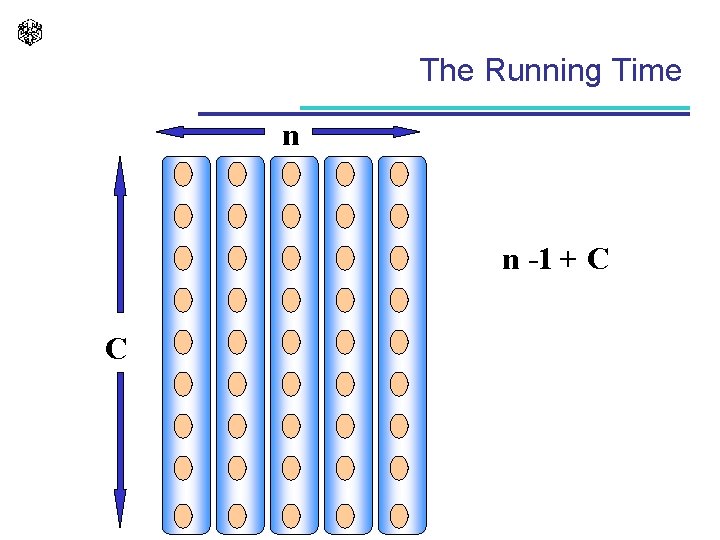
The Running Time n n -1 + C C

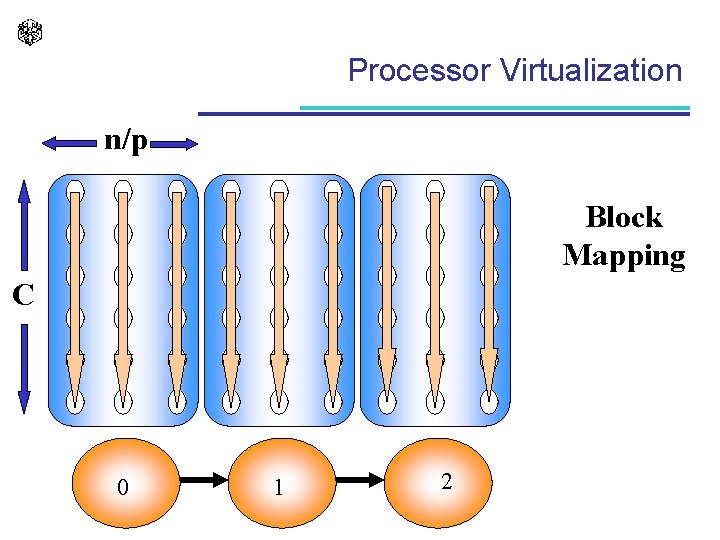
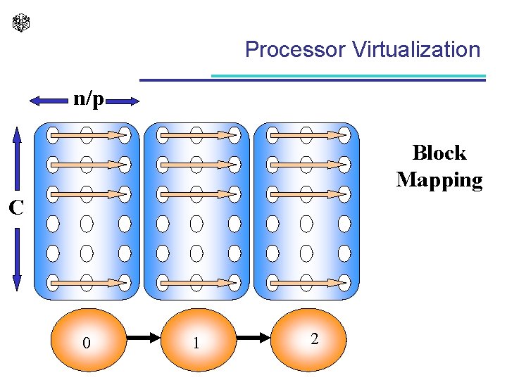
Processor Virtualization n/p Block Mapping C 0 1 2

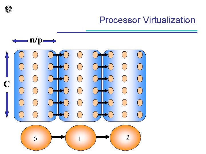
Processor Virtualization n/p Block Mapping C 0 1 2

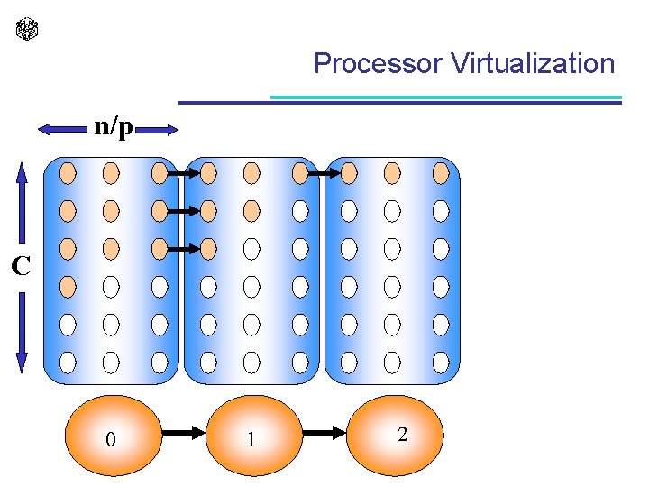
Processor Virtualization n/p C 0 1 2

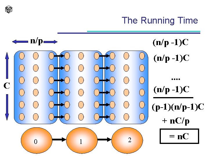
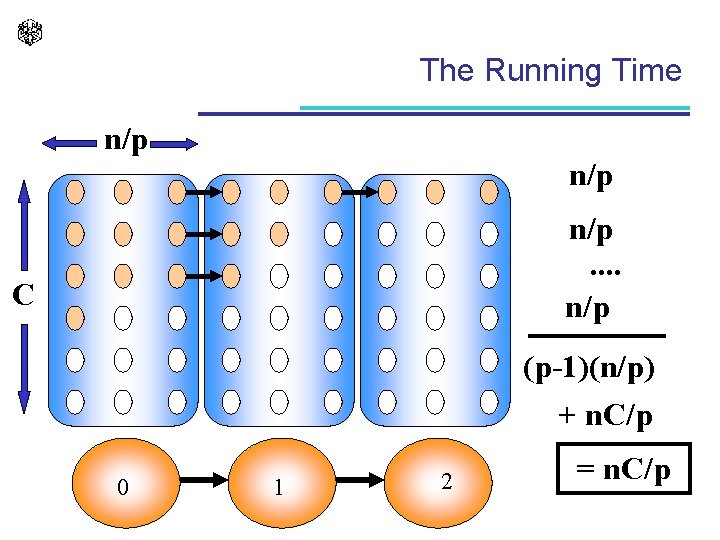
The Running Time n/p (n/p -1)C. . (n/p -1)C C (p-1)(n/p-1)C + n. C/p 0 1 2 = n. C

Processor Virtualization n/p C 0 1 2

The Running Time n/p n/p. . n/p C (p-1)(n/p) + n. C/p 0 1 2 = n. C/p

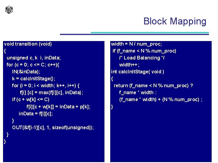
Block Mapping void transition (void) { unsigned c, k i, in. Data; for (c = 0; c <= C; c++){ IN(&in. Data); k = calc. Init. Stage(); for (i = 0; i < width; k++, i++) { f[i] [c] = max(f[i][c], in. Data); if (c + w[k] <= C) f[i][c + w[k]] = in. Data + p[k]; in. Data = f[i][c]; } OUT(&f[i-1][c], 1, sizeof(unsigned)); } } width = N / num_proc; if (f_name < N % num_proc) /* Load Balancing */ width++; int calc. Init. Stage( void ) { return (f_name < N % num_proc) ? f_name * width : (f_name * width) + (N % num_proc) ; }

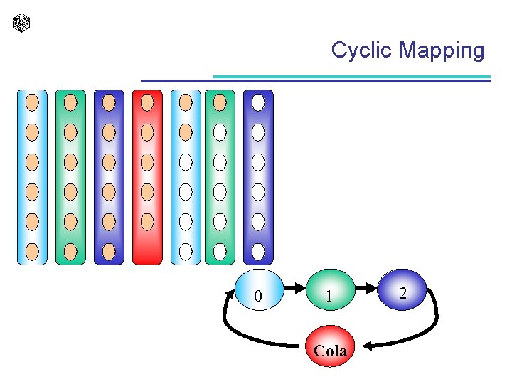
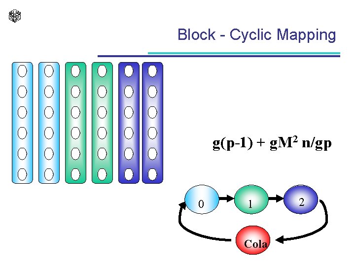
Cyclic Mapping 0 1 Cola 2

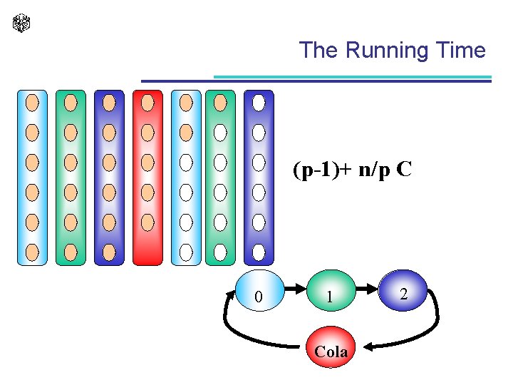
The Running Time (p-1)+ n/p C 0 1 Cola 2

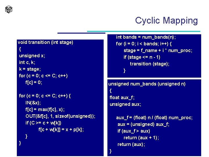
Cyclic Mapping void transition (int stage) { unsigned x; int c, k; k = stage; for (c = 0; c <= C; c++) f[c] = 0; for (c = 0; c <= C; c++) { IN(&x); f[c] = max(f[c], x); OUT(&f[c], 1, sizeof(unsigned)); if (C >= c + w[k]) f[c + w[k]] = x + p[k]; } } int bands = num_bands(n); for (i = 0; i < bands; i++) { stage = f_name + i * num_proc; if (stage <= n - 1) transition (stage); } unsigned num_bands (unsigned n) { float aux_f; unsigned aux; aux_f = (float) n / (float) num_proc; aux = (unsigned) aux_f; if (aux_f > aux) return (aux + 1); return (aux); }

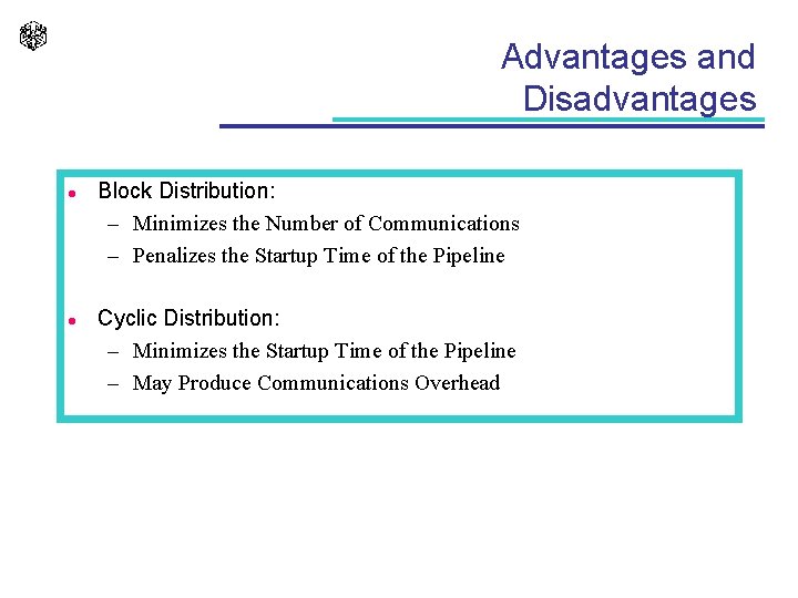
Advantages and Disadvantages l l Block Distribution: – Minimizes the Number of Communications – Penalizes the Startup Time of the Pipeline Cyclic Distribution: – Minimizes the Startup Time of the Pipeline – May Produce Communications Overhead

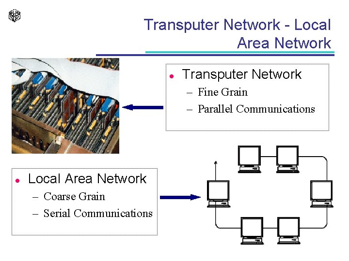
Transputer Network - Local Area Network l Transputer Network – Fine Grain – Parallel Communications l Local Area Network – Coarse Grain – Serial Communications

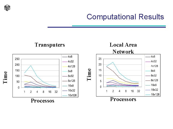
Computational Results Local Area Network Time Transputers Processors

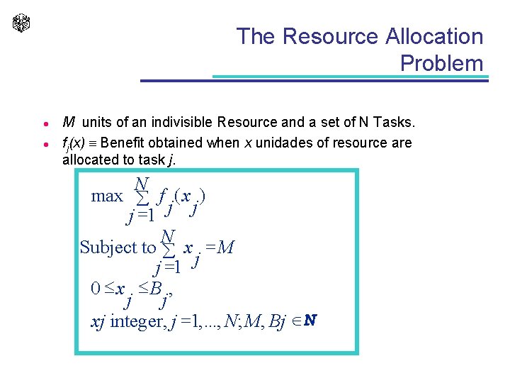
The Resource Allocation Problem l l M units of an indivisible Resource and a set of N Tasks. fj(x) Benefit obtained when x unidades of resource are allocated to task j. N max å f ( x ) j =1 j j N Subject to å x = M j =1 j 0 x B , j j xj integer, j =1, . . . , N; M, Bj ÎN

RAP- The Sequential Algorithm G[k][m] = max{G[k-1][m-i] + fk(i) / 0 i m } int rap_seq(void) { int i, k, m; for (m = 0; m <= M; n++) G[0][m] = 0; q = a; Q = b; for(k = 0; k < N; k++) { for(m = 0; m <= M; m++) { for (i = 0; i <= m; i++) G[k][m] = max{G[k][m], G[k-1][i] + f[k](m- i)}; } return G[N ][M]; } O(n. M 2)

RAP - The Parallel Algorithm . . Processor k . . . G[k-1][m] . . . . m. . 4: for( m = 0; m <= M; m++) 5: G[m] = 0; 6: k = stage; 7: for (m = 0; m <= M; m++) { 8: IN(&x); 9: G[m] = max(G[m], x + f(k-1, 0)); 10: OUT(&G[m], 1, sizeof(int)); 11: for (j = m + 1; j <= M; j++) 12: G[j] = max(G[j], x + f(k - 1, j - m)); 13: } /* for m. . . */ 14: } /* transition */ Processor k - 1 . . 1: void transition (int stage) 2: { 3: int m, j, x, k; G[k][m] = max{G[k-1][m-i] + fk(i) / 0 i m }

The Cray T 3 E l CRAY T 3 E – Shared Address Space – Three-Dimensional Toroidal Network

Block - Cyclic Mapping g(p-1) + g. M 2 n/gp 0 1 Cola 2

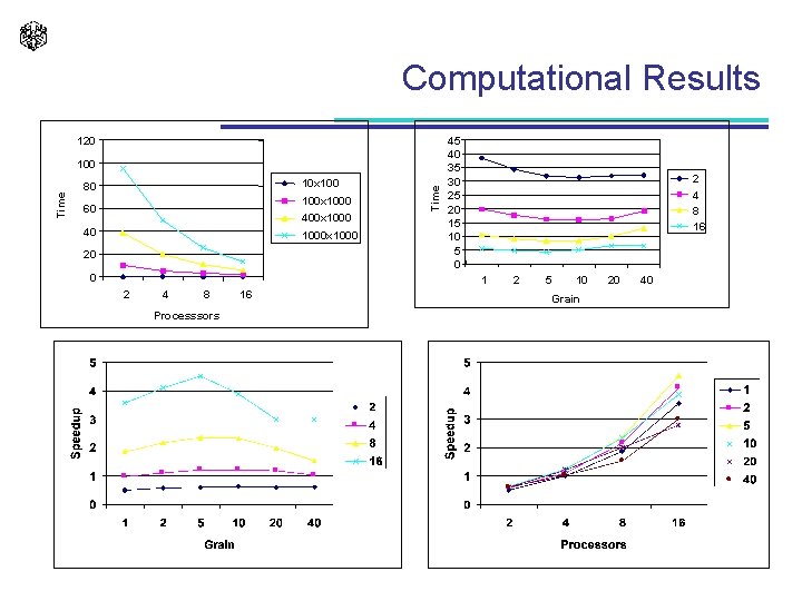
Computational Results 120 10 x 100 80 100 x 1000 60 400 x 1000 40 1000 x 1000 20 0 Time 100 45 40 35 30 25 20 15 10 5 0 2 4 8 16 1 2 4 8 Processsors 16 2 5 10 Grain 20 40

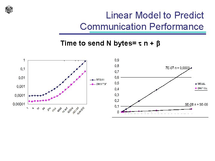
Linear Model to Predict Communication Performance Time to send N bytes= n + b

PAPI l l http: //icl. cs. utk. edu/projects/papi/ PAPI aims to provide the tool designer and application engineer with a consistent interface and methodology for use of the performance counter hardware found in most major microprocessors.

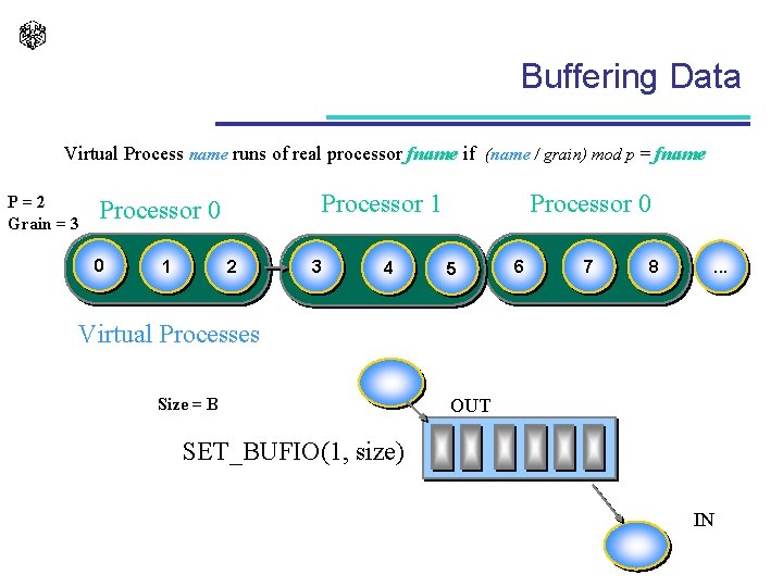
Buffering Data Virtual Process name runs of real processor fname if (name / grain) mod p = fname P=2 Grain = 3 Processor 1 Processor 0 0 1 2 3 4 Processor 0 5 6 7 8 . . . Virtual Processes Size = B OUT SET_BUFIO(1, size) IN

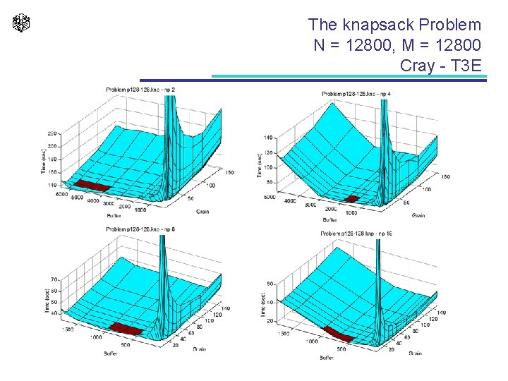
The knapsack Problem N = 12800, M = 12800 Cray - T 3 E

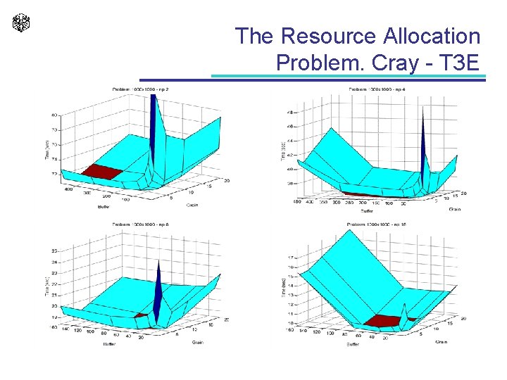
The Resource Allocation Problem. Cray - T 3 E

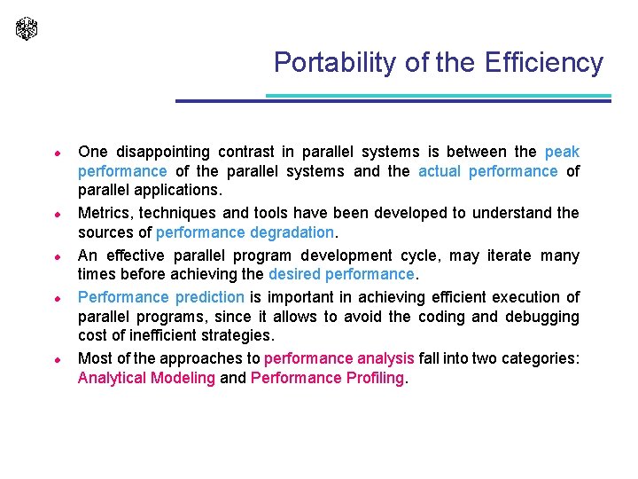
Portability of the Efficiency l l l One disappointing contrast in parallel systems is between the peak performance of the parallel systems and the actual performance of parallel applications. Metrics, techniques and tools have been developed to understand the sources of performance degradation. An effective parallel program development cycle, may iterate many times before achieving the desired performance. Performance prediction is important in achieving efficient execution of parallel programs, since it allows to avoid the coding and debugging cost of inefficient strategies. Most of the approaches to performance analysis fall into two categories: Analytical Modeling and Performance Profiling.

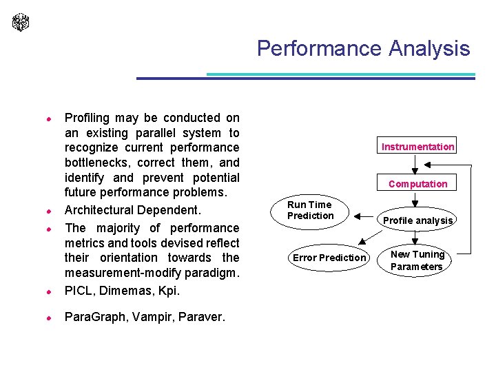
Performance Analysis l Profiling may be conducted on an existing parallel system to recognize current performance bottlenecks, correct them, and identify and prevent potential future performance problems. Architectural Dependent. The majority of performance metrics and tools devised reflect their orientation towards the measurement-modify paradigm. PICL, Dimemas, Kpi. l Para. Graph, Vampir, Paraver. l l l Instrumentation Computation Run Time Prediction Error Prediction Profile analysis New Tuning Parameters

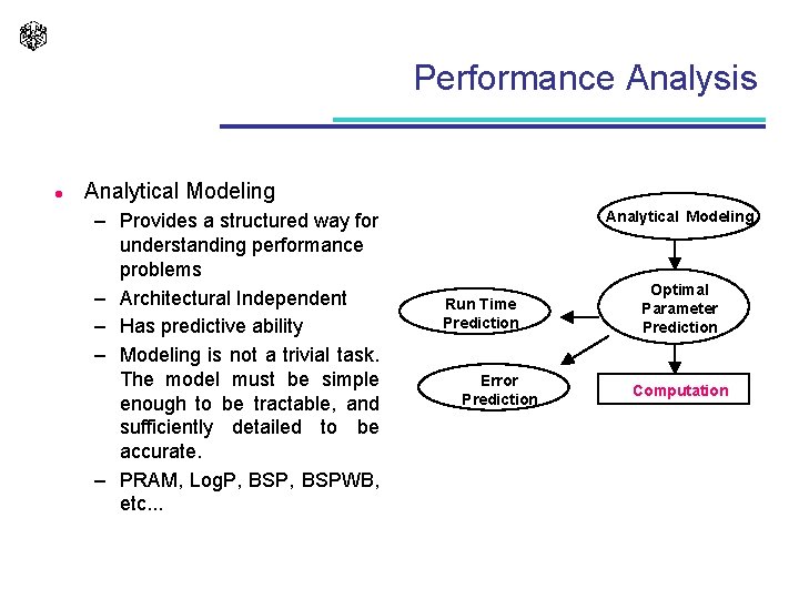
Performance Analysis l Analytical Modeling – Provides a structured way for understanding performance problems – Architectural Independent – Has predictive ability – Modeling is not a trivial task. The model must be simple enough to be tractable, and sufficiently detailed to be accurate. – PRAM, Log. P, BSPWB, etc. . . Analytical Modeling Run Time Prediction Error Prediction Optimal Parameter Prediction Computation

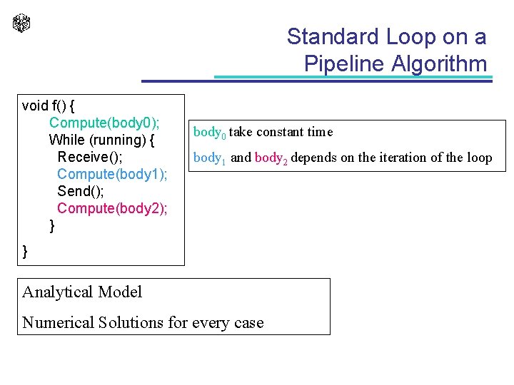
Standard Loop on a Pipeline Algorithm void f() { Compute(body 0); While (running) { Receive(); Compute(body 1); Send(); Compute(body 2); } body 0 take constant time body 1 and body 2 depends on the iteration of the loop } Analytical Model Numerical Solutions for every case

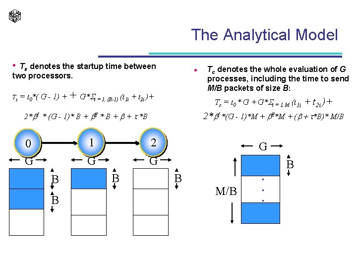
The Analytical Model • Ts denotes the startup time between two processors. Ts l = t 0*( G - 1) + + G* i = 1, (B-1) (t 1 i + t 2 i )+ Tc = t 0 * G + G* i = 1, M (t 1 i B B 1 2 G G B + t 2 i )+ 2*b. I *(G - 1)*M + b. E*M + (b + t*B)* M/B 2*b. I * (G - 1)* B + b. E * B + b + t *B 0 G Tc denotes the whole evaluation of G processes, including the time to send M/B packets of size B: G B B M/B . . .

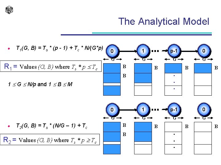
The Analytical Model l T 1(G, B) = Ts * (p - 1) + Tc * N/(G*p) 0 1 p-1 0 G G R 1 = Values (G, B) where Ts * p Tc B B 1 G N/p and 1 B M T 2(G, B) = Ts * (N/G – 1) + Tc R 2 = Values (G, B) where Ts * p Tc B . . . B l B 0 1 p-1 0 G G B B . . . B

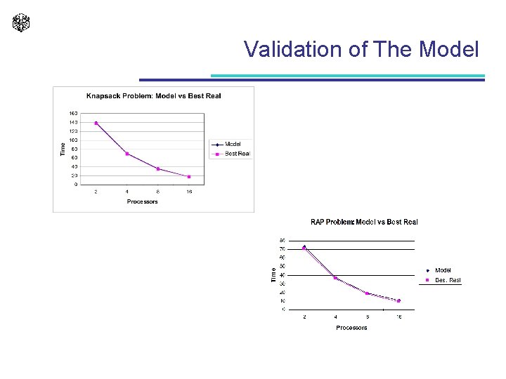
Validation of The Model

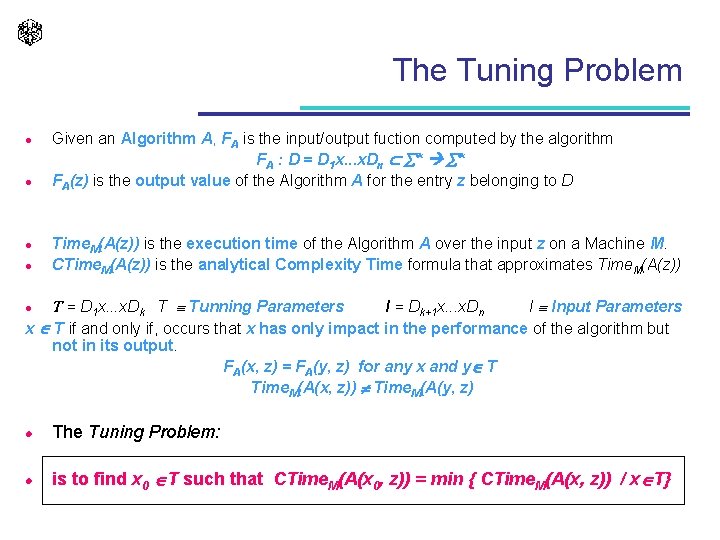
The Tuning Problem l l Given an Algorithm A, FA is the input/output fuction computed by the algorithm FA : D = D 1 x. . . x. Dn * * FA(z) is the output value of the Algorithm A for the entry z belonging to D Time. M(A(z)) is the execution time of the Algorithm A over the input z on a Machine M. CTime. M(A(z)) is the analytical Complexity Time formula that approximates Time. M(A(z)) T = D 1 x. . . x. Dk T Tunning Parameters I = Dk+1 x. . . x. Dn I Input Parameters x T if and only if, occurs that x has only impact in the performance of the algorithm but not in its output. FA(x, z) = FA(y, z) for any x and y T Time. M(A(x, z)) Time. M(A(y, z) l l The Tuning Problem: l is to find x 0 T such that CTime. M(A(x 0, z)) = min { CTime. M(A(x, z)) / x T}

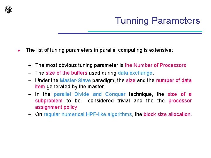
Tunning Parameters l The list of tuning parameters in parallel computing is extensive: – The most obvious tuning parameter is the Number of Processors. – The size of the buffers used during data exchange. – Under the Master-Slave paradigm, the size and the number of data item generated by the master. – In the parallel Divide and Conquer technique, the size of a subproblem to be considered trivial and the processor assignment policy. – On regular numerical HPF-like algorithms, the block size allocation.

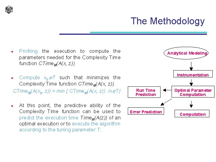
The Methodology l Profiling the execution to compute the parameters needed for the Complexity Time function CTime. M(A(x, z)). Compute x 0 T such that minimizes the Complexity Time function CTime. M(A(x, z)). CTime. M(A(x 0, z)) = min { CTime. M(A(x, z)) /x T} Analytical Modeling Instrumentation l l At this point, the predictive ability of the Complexity Time function can be used to predict the execution time Time. M(A(z)) of an optimal execution or to execute the algorithm according to the tuning parameter T. Run Time Prediction Error Prediction Optimal Parameter Computation

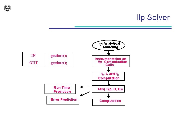
llp Solver llp Analytical Modeling IN gettime(); OUT gettime(); Instrumentation on llp Comunication Calls t 0, t 1 and t 2 Computation Run Time Prediction Error Prediction Min( T(p, G, B)) Computation

The MALLBA Infrastructure BA L L MA

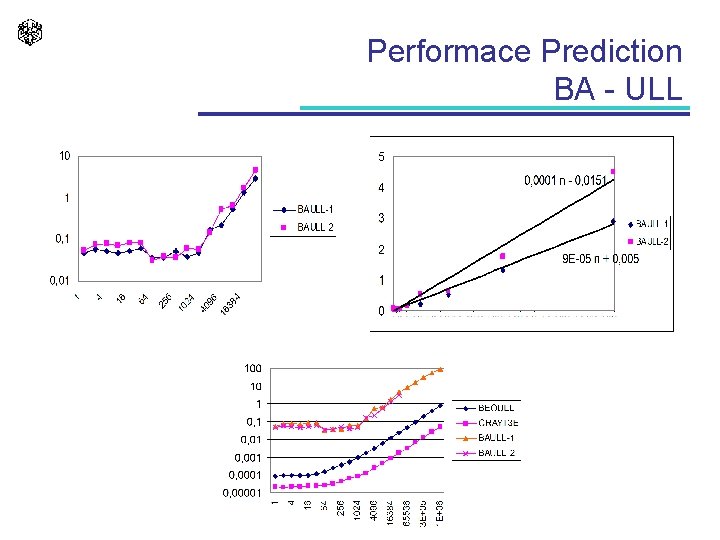
Performace Prediction BA - ULL

The MALLBA Project l Library for the resolution of combinatorial optimisation problems. – 3 types of resolution techniques: • Exact • Heuristic • Hybrid – 3 implementations: • Sequential • LAN • WAN l Goals: – Genericity

References l l l Willkinson B. , Allen M. Parallel Programming. Techniques and Applications Using Networkded Workstations and Parallel Computers. 1999. Prentice-Hall. Gropp W. , Lusk E. , Skjellum A. Using MPI. Portable Parallel Programming with the Message-Passing Interface. 1999. The MIT Press. Pacheco P. Parallel Programming with MPI. 1997. Morgan Kaufmann Publishers. Wu X. Performance Evaluation, Prediction and Visualization of Parallel Systems. nereida. deioc. ull. es