Introduction to Compu Cell 3 D Outline 1

Introduction to Compu. Cell 3 D Outline: 1. What is Compu. Cell 3 D? 2. Why use Compu. Cell 3 D? 3. Demo simulations 4. Glazier-Graner-Hogeweg (GGH) model – an overview 5. Compu. Cell 3 D architecture and terminology 6. XML 101 7. Building first Compu. Cell 3 D simulation 8. Visualization package – Compu. Cell Player 9. Python scripting inside Compu. Cell 3 D

What Is Compu. Cell 3 D? 1. Compu. Cell 3 D is a modeling environment used to build, test, run and visualize GGH-based simulations 2. Compu. Cell 3 D has built-in scripting language (Python) that allows users to quite easily write extension modules that are essential for building sophisticated biological models. 3. Compu. Cell 3 D thus is NOT a specialized software 4. Running Compu. Cell 3 D simulations DOES NOT recompilation 5. Compu. Cell 3 D model is described using Compu. Cell 3 D XML syntax and in the case of using Python language , a Python script(s) 6. Compu. Cell 3 D platform is distributed with a GUI front end – Compu. Cell Player or simply Player. The Player provides 2 - and 3 -D visualization capabilities. 7. Models developed by one Compu. Cell 3 D user can be “replayed” by another user regardless the operating system/hardware on which Compu. Cell is installed. 8. Compu. Cell 3 D is a cross platform application with Windows port being currently developed (due end of July 2007).

Why Use Compu. Cell 3 D? What Are the Alternatives? 1. Compu. Cell 3 D allows users to set up and run their simmulations within minutes, maybe hours. A typical development of a specialized GGH code takes orders of magnitudes longer time. 2. Compu. Cell 3 D simulations DO NOT need to be recompiled. If you want to change parameters (in XML or Python scripts) or logic (in Python scripts) you just make the changes and re-run the simulation. With hand-compiled simulations there is much more to do. Recompilation of every simulation is also error prone and often limits users to those who have significant programming background. 3. Compu. Cell 3 D is actively developed , maintained and supported. On www. compucell 3 d. org website users can download manuals, tutorials and developer documentation. Compu. Cell 3 D has approx. 10 releases each year. 4. Compu. Cell 3 D has many users around the world. This makes it easier to collaborate or exchange modules and results saving time spent on developing new model. 5. The Biocomplexity Institute organizes training workshops and mentorship programs. Those are great opportunities to visit Bloomington and learn biological modeling using Compu. Cell 3 D. For more info see www. compucell 3 d. org

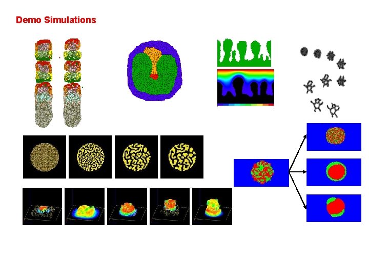
Demo Simulations

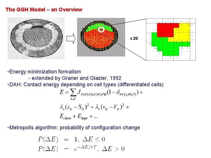
The GGH Model – an Overview x 20 • Energy minimization formalism - extended by Graner and Glazier, 1992 • DAH: Contact energy depending on cell types (differentiated cells) • Metropolis algorithm: probability of configuration change

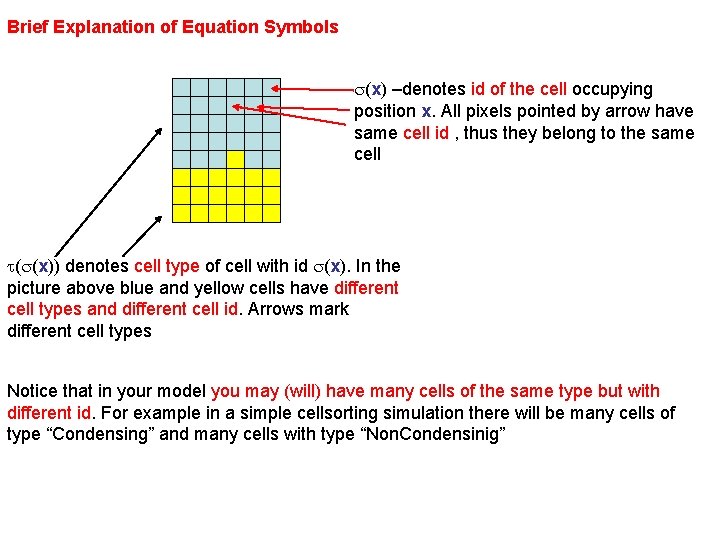
Brief Explanation of Equation Symbols s(x) –denotes id of the cell occupying position x. All pixels pointed by arrow have same cell id , thus they belong to the same cell t(s(x)) denotes cell type of cell with id s(x). In the picture above blue and yellow cells have different cell types and different cell id. Arrows mark different cell types Notice that in your model you may (will) have many cells of the same type but with different id. For example in a simple cellsorting simulation there will be many cells of type “Condensing” and many cells with type “Non. Condensinig”

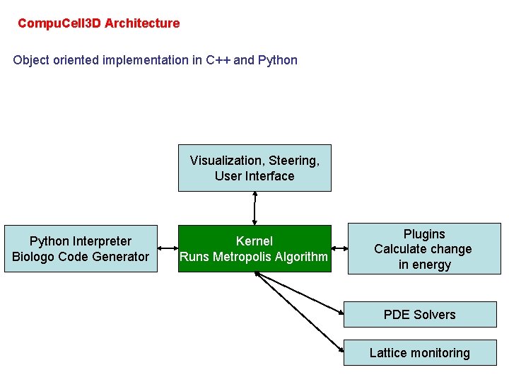
Compu. Cell 3 D Architecture Object oriented implementation in C++ and Python Visualization, Steering, User Interface Python Interpreter Biologo Code Generator Kernel Runs Metropolis Algorithm Plugins Calculate change in energy PDE Solvers Lattice monitoring

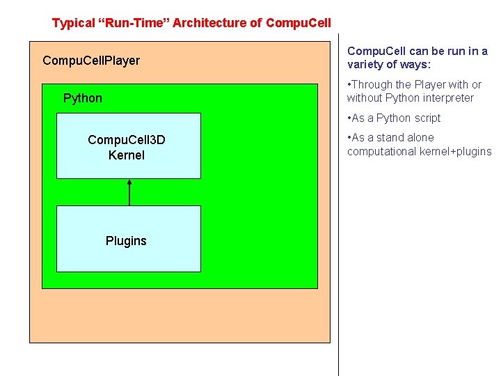
Typical “Run-Time” Architecture of Compu. Cell. Player Compu. Cell can be run in a variety of ways: • Through the Player with or without Python interpreter Python • As a Python script Compu. Cell 3 D Kernel Plugins • As a stand alone computational kernel+plugins

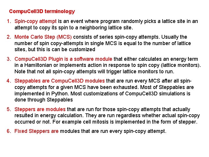
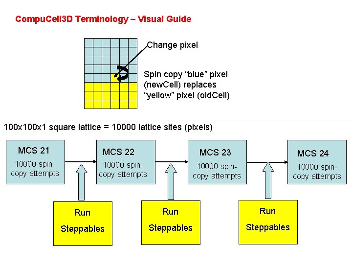
Compu. Cell 3 D terminology 1. Spin-copy attempt is an event where program randomly picks a lattice site in an attempt to copy its spin to a neighboring lattice site. 2. Monte Carlo Step (MCS) consists of series spin-copy attempts. Usually the number of spin copy-attempts in single MCS is equal to the number of lattice sites, but this is can be customized 3. Compu. Cell 3 D Plugin is a software module that either calculates an energy term in a Hamiltonian or implements action in response to spin copy (lattice monitors). Note that not all spin-copy attempts will trigger lattice monitors to run. 4. Steppables are Compu. Cell 3 D modules that are run every MCS after all spincopy attempts for a given MCS have been exhausted. Most of Steppables are implemented in Python. Most customizations of Compu. Cell 3 D simulations is done through Steppables 5. Steppers are modules that are run for those spin-copy attempts that actually resulted in energy calculation. They are run regardless whether actual spin-copy occurred or not. For example cell mitosis is implemented in the form of stepper. 6. Fixed Steppers are modules that are run every spin-copy attempt.

Compu. Cell 3 D Terminology – Visual Guide Change pixel Spin copy “blue” pixel (new. Cell) replaces “yellow” pixel (old. Cell) 100 x 1 square lattice = 10000 lattice sites (pixels) MCS 21 MCS 22 10000 spincopy attempts MCS 23 10000 spincopy attempts MCS 24 10000 spincopy attempts Run Run Steppables

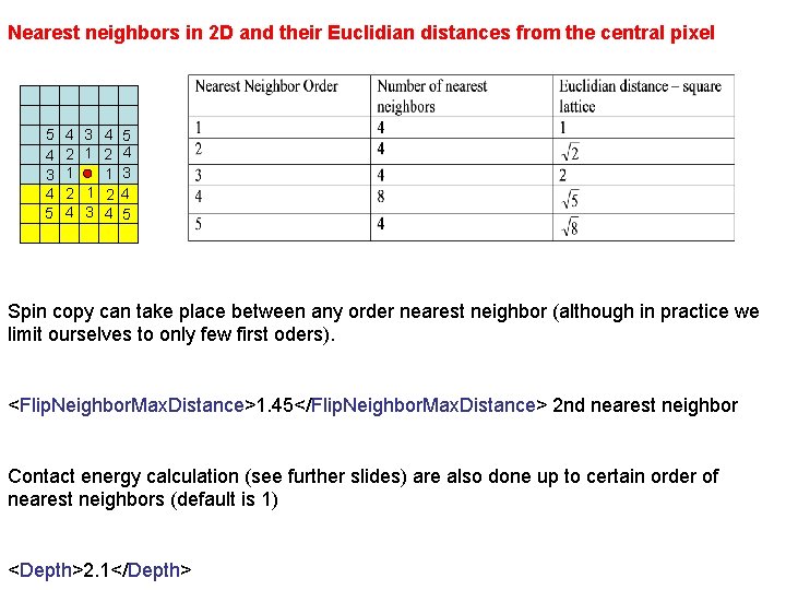
Nearest neighbors in 2 D and their Euclidian distances from the central pixel 5 4 3 4 5 4 2 1 2 4 3 4 5 1 2 4 1 3 1 2 4 3 4 5 Spin copy can take place between any order nearest neighbor (although in practice we limit ourselves to only few first oders). <Flip. Neighbor. Max. Distance>1. 45</Flip. Neighbor. Max. Distance> 2 nd nearest neighbor Contact energy calculation (see further slides) are also done up to certain order of nearest neighbors (default is 1) <Depth>2. 1</Depth>

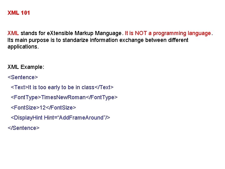
XML 101 XML stands for e. Xtensible Markup Manguage. It is NOT a programming language. Its main purpose is to standarize information exchange between different applications. XML Example: <Sentence> <Text>It is too early to be in class</Text> <Font. Type>Times. New. Roman</Font. Type> <Font. Size>12</Font. Size> <Display. Hint=“Add. Frame. Around”/> </Sentence>

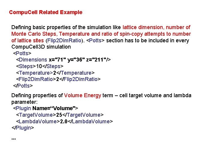
Compu. Cell Related Example Defining basic properties of the simulation like lattice dimension, number of Monte Carlo Steps, Temperature and ratio of spin-copy attempts to number of lattice sites (Flip 2 Dim. Ratio). <Potts> section has to be included in every Compu. Cell 3 D simulation <Potts> <Dimensions x="71" y="36" z="211"/> <Steps>10</Steps> <Temperature>2</Temperature> <Flip 2 Dim. Ratio>2</Flip 2 Dim. Ratio> </Potts> Defining properties of Volume Energy term – cell target volume and lambda parameter: <Plugin Name=“Volume"> <Target. Volume>25</Target. Volume> <Lambda. Volume>2. 0</Lambda. Volume> </Plugin>. . .

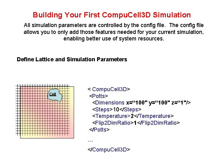
Building Your First Compu. Cell 3 D Simulation All simulation parameters are controlled by the config file. The config file allows you to only add those features needed for your current simulation, enabling better use of system resources. Define Lattice and Simulation Parameters Cell < Compu. Cell 3 D> <Potts> <Dimensions x=“ 100" y=“ 100" z=“ 1"/> <Steps>10</Steps> <Temperature>2</Temperature> <Flip 2 Dim. Ratio>1</Flip 2 Dim. Ratio> </Potts> … </Compu. Cell 3 D>

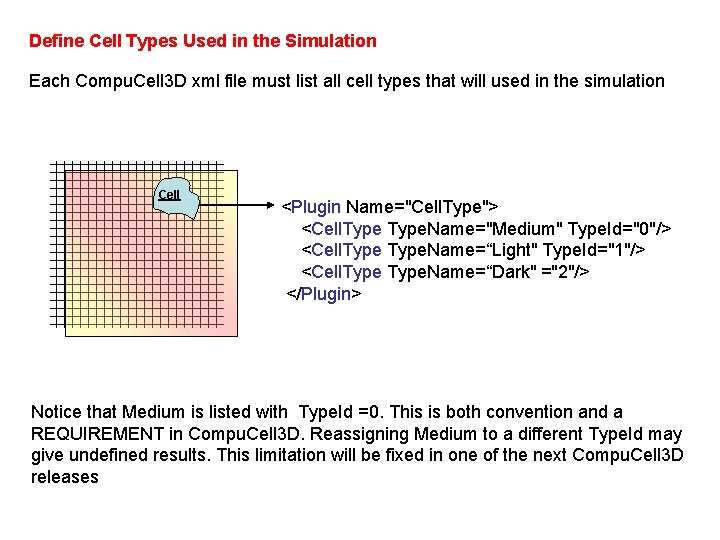
Define Cell Types Used in the Simulation Each Compu. Cell 3 D xml file must list all cell types that will used in the simulation Cell <Plugin Name="Cell. Type"> <Cell. Type. Name="Medium" Type. Id="0"/> <Cell. Type. Name=“Light" Type. Id="1"/> <Cell. Type. Name=“Dark" ="2"/> </Plugin> Notice that Medium is listed with Type. Id =0. This is both convention and a REQUIREMENT in Compu. Cell 3 D. Reassigning Medium to a different Type. Id may give undefined results. This limitation will be fixed in one of the next Compu. Cell 3 D releases

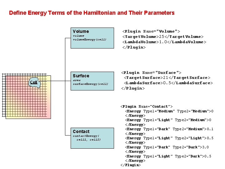
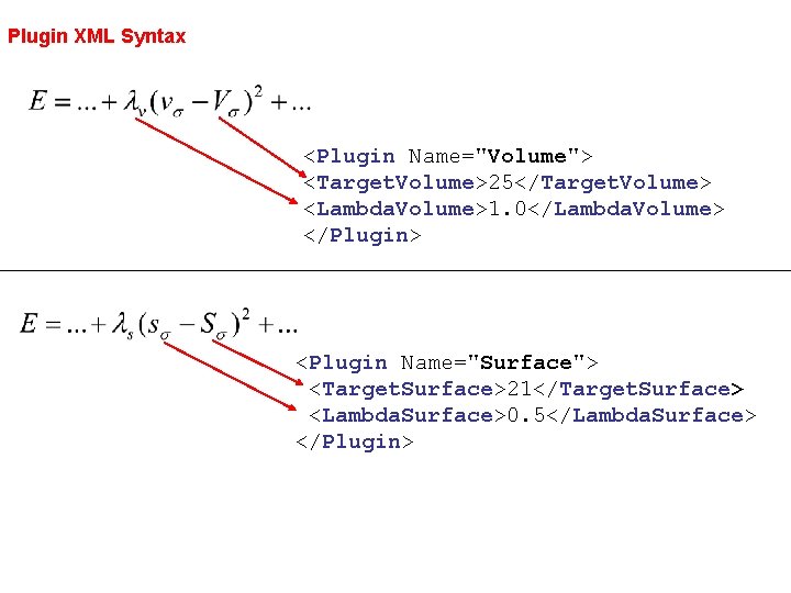
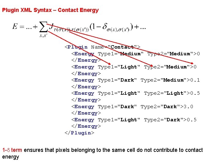
Define Energy Terms of the Hamiltonian and Their Parameters Volume volume. Energy(cell) Surface Cell area surface. Energy(cell) Contact contact. Energy( cell 1, cell 2) <Plugin Name="Volume"> <Target. Volume>25</Target. Volume> <Lambda. Volume>1. 0</Lambda. Volume> </Plugin> <Plugin Name="Surface"> <Target. Surface>21</Target. Surface> <Lambda. Surface>0. 5</Lambda. Surface> </Plugin> <Plugin Name="Contact"> <Energy Type 1="Medium" Type 2="Medium">0 </Energy> <Energy Type 1="Light" Type 2="Medium">0 </Energy> <Energy Type 1="Dark" Type 2="Medium">0. 1 </Energy> <Energy Type 1="Light" Type 2="Light">0. 5 </Energy> <Energy Type 1="Dark" Type 2="Dark">3. 0 </Energy> <Energy Type 1="Light" Type 2="Dark">0. 5 </Energy> </Plugin>

Plugin XML Syntax <Plugin Name="Volume"> <Target. Volume>25</Target. Volume> <Lambda. Volume>1. 0</Lambda. Volume> </Plugin> <Plugin Name="Surface"> <Target. Surface>21</Target. Surface> <Lambda. Surface>0. 5</Lambda. Surface> </Plugin>

Plugin XML Syntax – Contact Energy <Plugin Name="Contact"> <Energy Type 1="Medium" Type 2="Medium">0 </Energy> <Energy Type 1="Light" Type 2="Medium">0 </Energy> <Energy Type 1="Dark" Type 2="Medium">0. 1 </Energy> <Energy Type 1="Light" Type 2="Light">0. 5 </Energy> <Energy Type 1="Dark" Type 2="Dark">3. 0 </Energy> <Energy Type 1="Light" Type 2="Dark">0. 5 </Energy> </Plugin> 1 -d term ensures that pixels belonging to the same cell do not contribute to contact energy

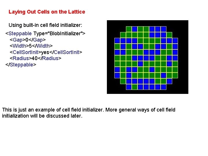
Laying Out Cells on the Lattice Using built-in cell field initializer: <Steppable Type="Blob. Initializer"> <Gap>0</Gap> <Width>5</Width> <Cell. Sort. Init>yes</Cell. Sort. Init> <Radius>40</Radius> </Steppable> This is just an example of cell field initializer. More general ways of cell field initialization will be discussed later.

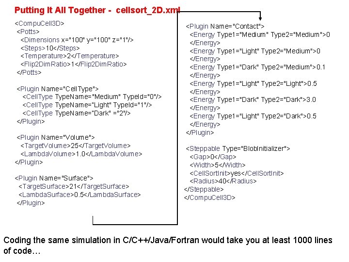
Putting It All Together - cellsort_2 D. xml <Compu. Cell 3 D> <Potts> <Dimensions x="100" y="100" z="1"/> <Steps>10</Steps> <Temperature>2</Temperature> <Flip 2 Dim. Ratio>1</Flip 2 Dim. Ratio> </Potts> <Plugin Name="Cell. Type"> <Cell. Type. Name="Medium" Type. Id="0"/> <Cell. Type. Name=“Light" Type. Id="1"/> <Cell. Type. Name=“Dark" ="2"/> </Plugin> <Plugin Name="Volume"> <Target. Volume>25</Target. Volume> <Lambda. Volume>1. 0</Lambda. Volume> </Plugin> <Plugin Name="Surface"> <Target. Surface>21</Target. Surface> <Lambda. Surface>0. 5</Lambda. Surface> </Plugin> <Plugin Name="Contact"> <Energy Type 1="Medium" Type 2="Medium">0 </Energy> <Energy Type 1="Light" Type 2="Medium">0 </Energy> <Energy Type 1="Dark" Type 2="Medium">0. 1 </Energy> <Energy Type 1="Light" Type 2="Light">0. 5 </Energy> <Energy Type 1="Dark" Type 2="Dark">3. 0 </Energy> <Energy Type 1="Light" Type 2="Dark">0. 5 </Energy> </Plugin> <Steppable Type="Blob. Initializer"> <Gap>0</Gap> <Width>5</Width> <Cell. Sort. Init>yes</Cell. Sort. Init> <Radius>40</Radius> </Steppable> </Compu. Cell 3 D> Coding the same simulation in C/C++/Java/Fortran would take you at least 1000 lines of code…

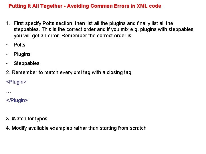
Putting It All Together - Avoiding Common Errors in XML code 1. First specify Potts section, then list all the plugins and finally list all the steppables. This is the correct order and if you mix e. g. plugins with steppables you will get an error. Remember the correct order is • Potts • Plugins • Steppables 2. Remember to match every xml tag with a closing tag <Plugin> … </Plugin> 3. Watch for typos 4. Modify available examples rather than starting from scratch

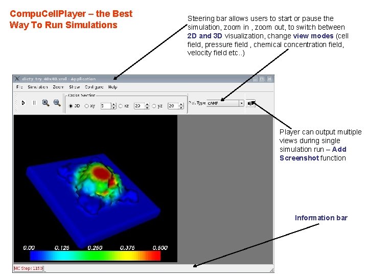
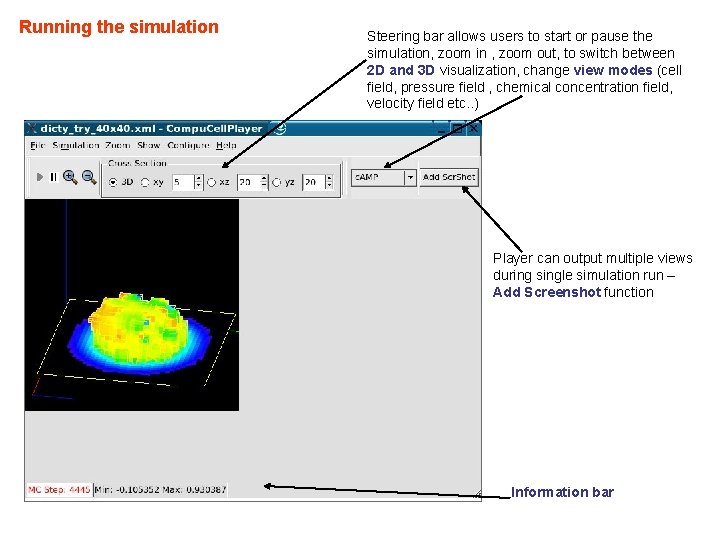
Compu. Cell. Player – the Best Way To Run Simulations Steering bar allows users to start or pause the simulation, zoom in , zoom out, to switch between 2 D and 3 D visualization, change view modes (cell field, pressure field , chemical concentration field, velocity field etc. . ) Player can output multiple views during single simulation run – Add Screenshot function Information bar

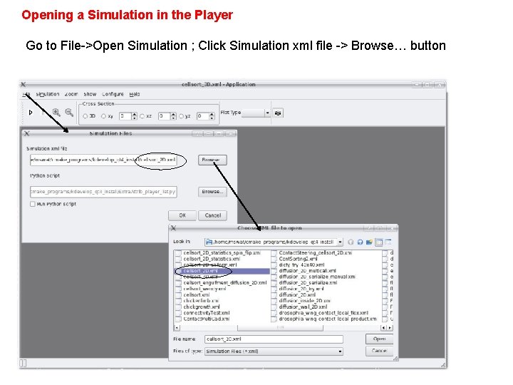
Opening a Simulation in the Player Go to File->Open Simulation ; Click Simulation xml file -> Browse… button

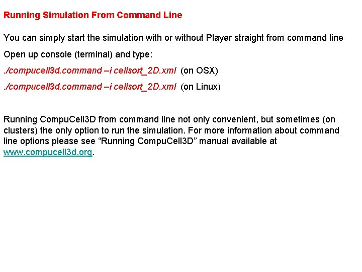
Running Simulation From Command Line You can simply start the simulation with or without Player straight from command line Open up console (terminal) and type: . /compucell 3 d. command –i cellsort_2 D. xml (on OSX). /compucell 3 d. command –i cellsort_2 D. xml (on Linux) Running Compu. Cell 3 D from command line not only convenient, but sometimes (on clusters) the only option to run the simulation. For more information about command line options please see “Running Compu. Cell 3 D” manual available at www. compucell 3 d. org.

Running the Simulation • After typing the XML file in your favorite editor all you need to do to run the simulation is to open the XML file in the Player and hit “Play” button. • Screenshots from the simulations are automatically stored in the directory with name composed of simulation file name and a time at which simulation was started • As you can see this setting Compu. Cell 3 D simulation was reasonably simple. • It is quite likely that if you were to code entire simulation in C/C++/Java etc. you would need much more time. • We hope that now you understand why using Compu. Cell 3 D saves you a lot of time and allows you to concentrate on biological modeling and not on writing low level computer code. • During last year we have improved Compu. Cell 3 D performance so that it is on par with hand-written code. Yet, if you really to have the fastest GGH code in the world you should write code your own simulation directly in C or even better in assembly language. Before you do it, make sure you want to spend time rewriting the code that already exist. We hope you will enjoy Compu. Cell 3 D and for more information please visit www. compucell 3 d. org.

Capabilities of Compu. Cell. Player • Provides wide range of visualization - cell field plots, concentration plots, vector field plots in both 2 - and 3 -D • Allows to store multiple lattice views in a single run. For example users can store multiple projections of the cell lattice, concentration fields, various 3 D views etc… in a single run. • Can be run in GUI and silent mode (i. e. without displaying GUI but still saving screenshots) • Is ready to be used on clusters that do not have X-server installed. This feature is essential for doing “production runs” of your simulations. • Concentration fields and vector fields initialized from Python level can easily be displayed in the Player • Configurable from XML level for those users who prefer typing to clicking

Compu. Cell Player 101

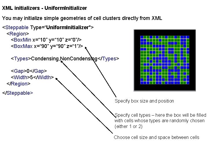
XML initializers - Uniform. Initializer You may initialize simple geometries of cell clusters directly from XML <Steppable Type=“Uniform. Initializer"> <Region> <Box. Min x=“ 10” y=“ 10” z=“ 0”/> <Box. Max x=“ 90” y=“ 90” z=“ 1”/> <Types>Condensing, Non. Condensing</Types> <Gap>0</Gap> <Width>5</Width> </Region> </Steppable> Specify box size and position Specify cell types – here the box will be filled with cells whose types are randomly chosen (either 1 or 2) Choose cell size and space between cells

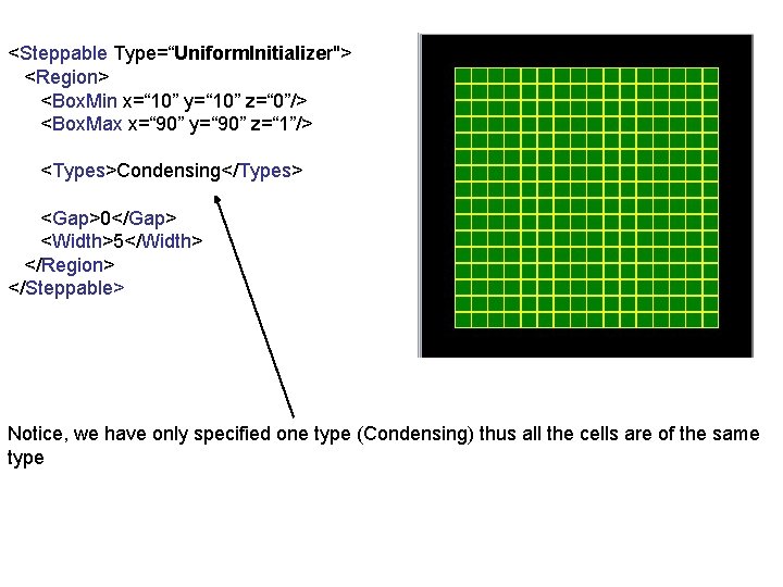
<Steppable Type=“Uniform. Initializer"> <Region> <Box. Min x=“ 10” y=“ 10” z=“ 0”/> <Box. Max x=“ 90” y=“ 90” z=“ 1”/> <Types>Condensing</Types> <Gap>0</Gap> <Width>5</Width> </Region> </Steppable> Notice, we have only specified one type (Condensing) thus all the cells are of the same type

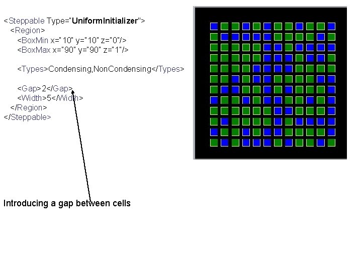
<Steppable Type=“Uniform. Initializer"> <Region> <Box. Min x=“ 10” y=“ 10” z=“ 0”/> <Box. Max x=“ 90” y=“ 90” z=“ 1”/> <Types>Condensing, Non. Condensing</Types> <Gap>2</Gap> <Width>5</Width> </Region> </Steppable> Introducing a gap between cells

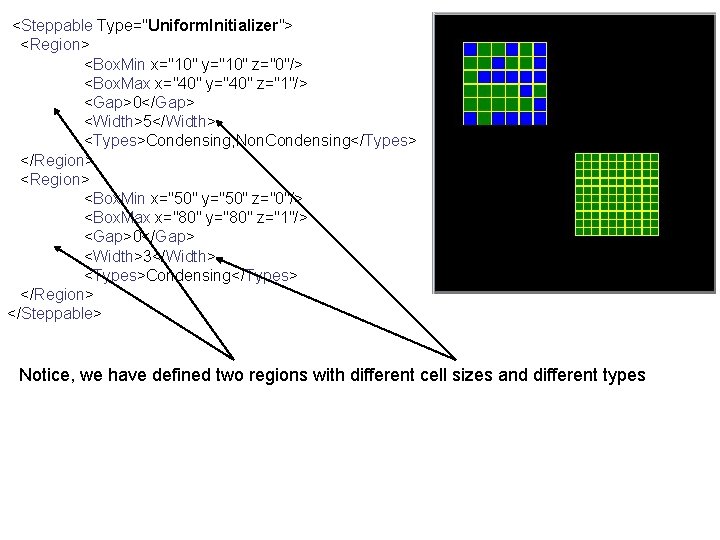
<Steppable Type="Uniform. Initializer"> <Region> <Box. Min x="10" y="10" z="0"/> <Box. Max x="40" y="40" z="1"/> <Gap>0</Gap> <Width>5</Width> <Types>Condensing, Non. Condensing</Types> </Region> <Box. Min x="50" y="50" z="0"/> <Box. Max x="80" y="80" z="1"/> <Gap>0</Gap> <Width>3</Width> <Types>Condensing</Types> </Region> </Steppable> Notice, we have defined two regions with different cell sizes and different types

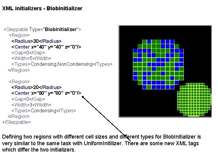
XML initializers - Blob. Initializer <Steppable Type="Blob. Initializer"> <Region> <Radius>30</Radius> <Center x="40" y="40" z="0"/> <Gap>0</Gap> <Width>5</Width> <Types>Condensing, Non. Condensing</Types> </Region> <Radius>20</Radius> <Center x="80" y="80" z="0"/> <Gap>0</Gap> <Width>3</Width> <Types>Condensing</Types> </Region> </Steppable> Defining two regions with different cell sizes and different types for Blob. Initializer is very similar to the same task with Uniform. Initilizer. There are some new XML tags which differ the two initializers.

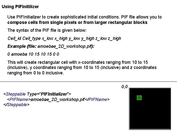
Using PIFInitilizer Use PIFInitializer to create sophisticated initial conditions. PIF file allows you to compose cells from single pixels or from larger rectangular blocks The syntax of the PIF file is given below: Cell_id Cell_type x_low x_high y_low y_high z_low z_high Example (file: amoebae_2 D_workshop. pif): 0 amoeba 10 15 0 0 This will create rectangular cell with x-coordinates ranging from 10 to 15 (inclusive), y coordinates ranging from 10 to 15 (inclusive) and z coordinates ranging from 0 to 0 inclusive. 0, 0 <Steppable Type="PIFInitializer"> <PIFName>amoebae_2 D_workshop. pif</PIFName> </Steppable>

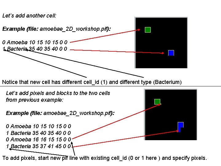
Let’s add another cell: Example (file: amoebae_2 D_workshop. pif): 0 Amoeba 10 15 0 0 1 Bacteria 35 40 0 0 Notice that new cell has different cell_id (1) and different type (Bacterium) Let’s add pixels and blocks to the two cells from previous example: Example (file: amoebae_2 D_workshop. pif): 0 Amoeba 10 15 0 0 1 Bacteria 35 40 0 0 0 Amoeba 16 16 15 15 0 0 1 Bacteria 35 37 41 45 0 0 To add pixels, start new pif line with existing cell_id (0 or 1 here ) and specify pixels.

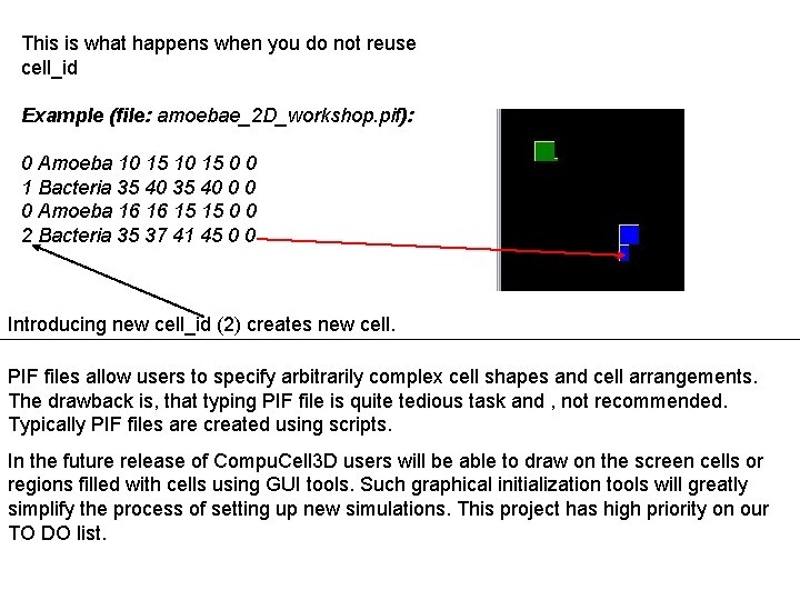
This is what happens when you do not reuse cell_id Example (file: amoebae_2 D_workshop. pif): 0 Amoeba 10 15 0 0 1 Bacteria 35 40 0 0 0 Amoeba 16 16 15 15 0 0 2 Bacteria 35 37 41 45 0 0 Introducing new cell_id (2) creates new cell. PIF files allow users to specify arbitrarily complex cell shapes and cell arrangements. The drawback is, that typing PIF file is quite tedious task and , not recommended. Typically PIF files are created using scripts. In the future release of Compu. Cell 3 D users will be able to draw on the screen cells or regions filled with cells using GUI tools. Such graphical initialization tools will greatly simplify the process of setting up new simulations. This project has high priority on our TO DO list.

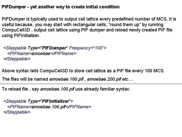
PIFDumper - yet another way to create initial condition PIFDumper is typically used to output cell lattice every predefined number of MCS. It is useful because, you may start with rectangular cells, “round them up” by running Compu. Cell 3 D , output cell lattice using PIF dumper and reload newly created PIF file using PIFInitializer. <Steppable Type="PIFDumper“ Frequency=“ 100”> <PIFName>amoebae</PIFName> </Steppable> Above syntax tells Compu. Cell 3 D to store cell lattice as a PIF file every 100 MCS. The files will be named amoebae. 100. pif , amoebae. 200. pif etc… To reload file , say amoebae. 100. pif use already familiar syntax: <Steppable Type="PIFInitializer"> <PIFName>amoebae. 100. pif</PIFName> </Steppable>

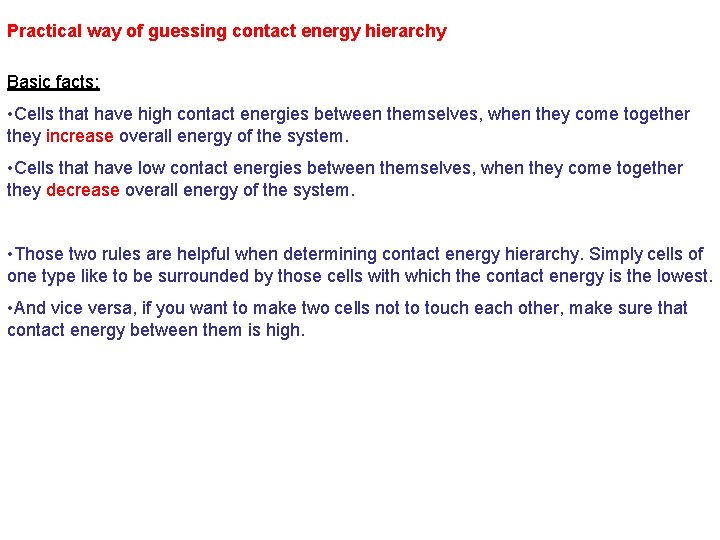
Practical way of guessing contact energy hierarchy Basic facts: • Cells that have high contact energies between themselves, when they come together they increase overall energy of the system. • Cells that have low contact energies between themselves, when they come together they decrease overall energy of the system. • Those two rules are helpful when determining contact energy hierarchy. Simply cells of one type like to be surrounded by those cells with which the contact energy is the lowest. • And vice versa, if you want to make two cells not to touch each other, make sure that contact energy between them is high.

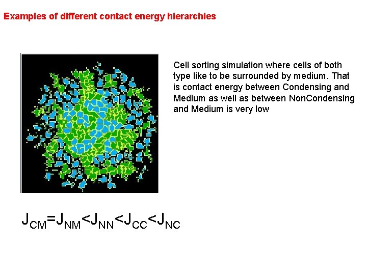
Examples of different contact energy hierarchies Cell sorting simulation where cells of both type like to be surrounded by medium. That is contact energy between Condensing and Medium as well as between Non. Condensing and Medium is very low JCM=JNM<JNN<JCC<JNC

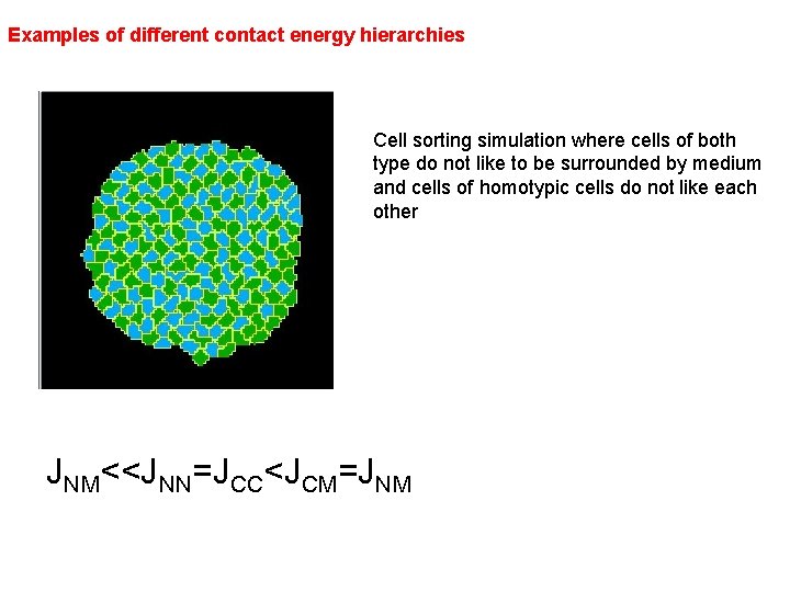
Examples of different contact energy hierarchies Cell sorting simulation where cells of both type do not like to be surrounded by medium and cells of homotypic cells do not like each other JNM<<JNN=JCC<JCM=JNM

Chemotaxis Basic facts • Chemotaxis is defined as cell motion induced by a presence (gradient) of a chemical. • In GGH formalism chemotaxis is implemented as a spin copy bias which depends on chemical gradient. • Chemotaxis was first introduced to GGH formalism by Paulien Hogeweg from University of Utrecht, Netherlands • In Compu. Cell 3 D Chemotaxis plugin provides wide range of options to support different modes of chemotaxis. • Chemotaxis plugin requires the presence of at least one concentration field. The fields can be inserted into Compu. Cell 3 D simulation by means PDE solvers or can be created, initialized and managed explicitly from the Python level

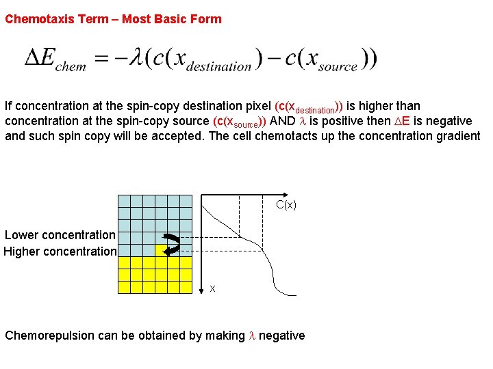
Chemotaxis Term – Most Basic Form If concentration at the spin-copy destination pixel (c(xdestination)) is higher than concentration at the spin-copy source (c(xsource)) AND l is positive then DE is negative and such spin copy will be accepted. The cell chemotacts up the concentration gradient C(x) Lower concentration Higher concentration x Chemorepulsion can be obtained by making l negative

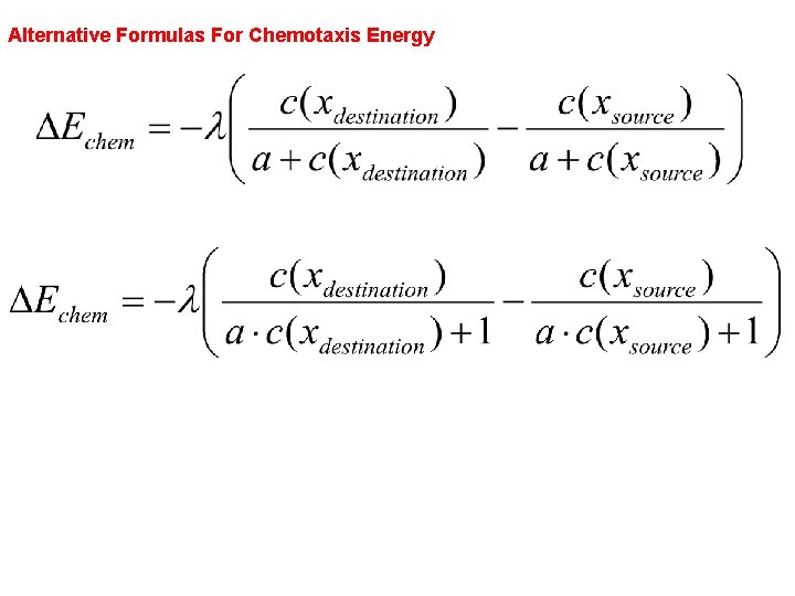
Alternative Formulas For Chemotaxis Energy

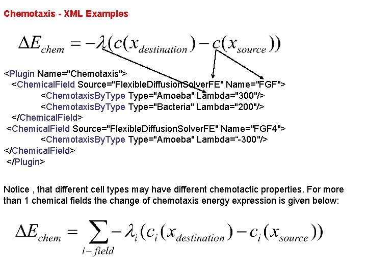
Chemotaxis - XML Examples <Plugin Name="Chemotaxis"> <Chemical. Field Source="Flexible. Diffusion. Solver. FE" Name="FGF"> <Chemotaxis. By. Type="Amoeba" Lambda="300"/> <Chemotaxis. By. Type="Bacteria" Lambda="200"/> </Chemical. Field> <Chemical. Field Source="Flexible. Diffusion. Solver. FE" Name="FGF 4"> <Chemotaxis. By. Type="Amoeba" Lambda=“-300"/> </Chemical. Field> </Plugin> Notice , that different cell types may have different chemotactic properties. For more than 1 chemical fields the change of chemotaxis energy expression is given below:

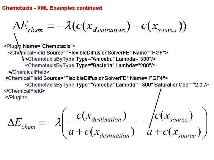
Chemotaxis - XML Examples continued <Plugin Name="Chemotaxis"> <Chemical. Field Source="Flexible. Diffusion. Solver. FE" Name="FGF"> <Chemotaxis. By. Type="Amoeba" Lambda="300"/> <Chemotaxis. By. Type="Bacteria" Lambda="200"/> </Chemical. Field> <Chemical. Field Source="Flexible. Diffusion. Solver. FE" Name="FGF 4"> <Chemotaxis. By. Type="Amoeba" Lambda=“-300“ Saturation. Coef=“ 2. 0”/> </Chemical. Field> </Plugin>

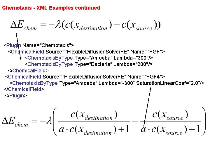
Chemotaxis - XML Examples continued <Plugin Name="Chemotaxis"> <Chemical. Field Source="Flexible. Diffusion. Solver. FE" Name="FGF"> <Chemotaxis. By. Type="Amoeba" Lambda="300"/> <Chemotaxis. By. Type="Bacteria" Lambda="200"/> </Chemical. Field> <Chemical. Field Source="Flexible. Diffusion. Solver. FE" Name="FGF 4"> <Chemotaxis. By. Type="Amoeba" Lambda=“-300“ Saturation. Linear. Coef=“ 2. 0”/> </Chemical. Field> </Plugin>

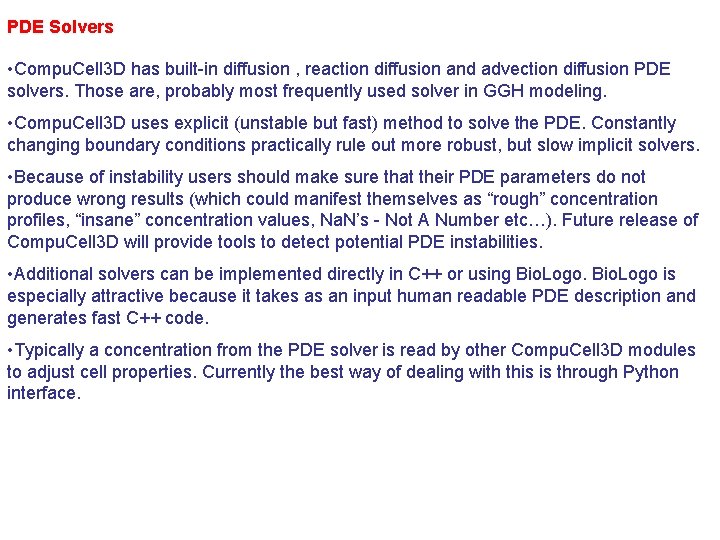
PDE Solvers • Compu. Cell 3 D has built-in diffusion , reaction diffusion and advection diffusion PDE solvers. Those are, probably most frequently used solver in GGH modeling. • Compu. Cell 3 D uses explicit (unstable but fast) method to solve the PDE. Constantly changing boundary conditions practically rule out more robust, but slow implicit solvers. • Because of instability users should make sure that their PDE parameters do not produce wrong results (which could manifest themselves as “rough” concentration profiles, “insane” concentration values, Na. N’s - Not A Number etc…). Future release of Compu. Cell 3 D will provide tools to detect potential PDE instabilities. • Additional solvers can be implemented directly in C++ or using Bio. Logo is especially attractive because it takes as an input human readable PDE description and generates fast C++ code. • Typically a concentration from the PDE solver is read by other Compu. Cell 3 D modules to adjust cell properties. Currently the best way of dealing with this is through Python interface.

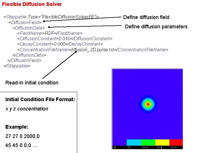
Flexible Diffusion Solver <Steppable Type="Flexible. Diffusion. Solver. FE"> Define diffusion field <Diffusion. Field> Define diffusion parameters <Diffusion. Data> <Field. Name>FGF</Field. Name> <Diffusion. Constant>0. 010</Diffusion. Constant> <Decay. Constant>0. 000</Decay. Constant> <Concentration. File. Name>diffusion_2 D. pulse. txt</Concentration. File. Name> </Diffusion. Data> </Diffusion. Field> </Steppable> Read-in initial condition Initial Condition File Format: x y z concentration Example: 27 27 0 2000. 0 45 45 0 0. 0 …

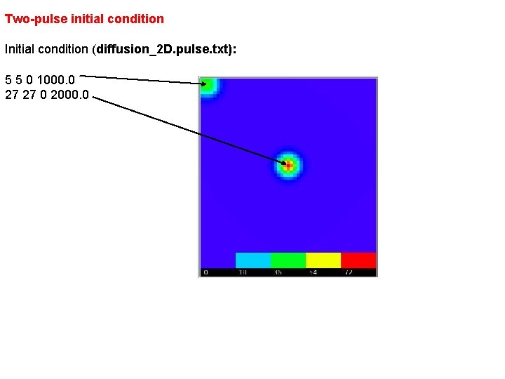
Two-pulse initial condition Initial condition (diffusion_2 D. pulse. txt): 5 5 0 1000. 0 27 27 0 2000. 0

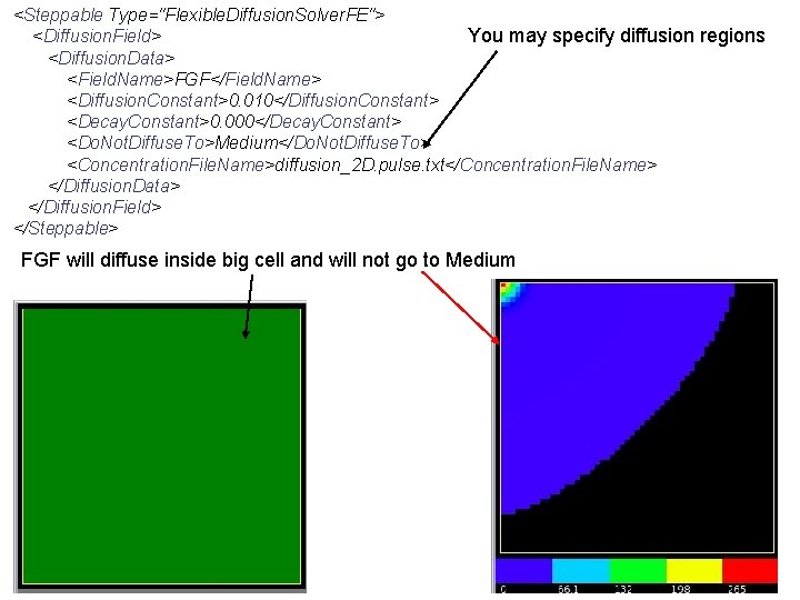
<Steppable Type="Flexible. Diffusion. Solver. FE"> <Diffusion. Field> You may specify diffusion regions <Diffusion. Data> <Field. Name>FGF</Field. Name> <Diffusion. Constant>0. 010</Diffusion. Constant> <Decay. Constant>0. 000</Decay. Constant> <Do. Not. Diffuse. To>Medium</Do. Not. Diffuse. To> <Concentration. File. Name>diffusion_2 D. pulse. txt</Concentration. File. Name> </Diffusion. Data> </Diffusion. Field> </Steppable> FGF will diffuse inside big cell and will not go to Medium

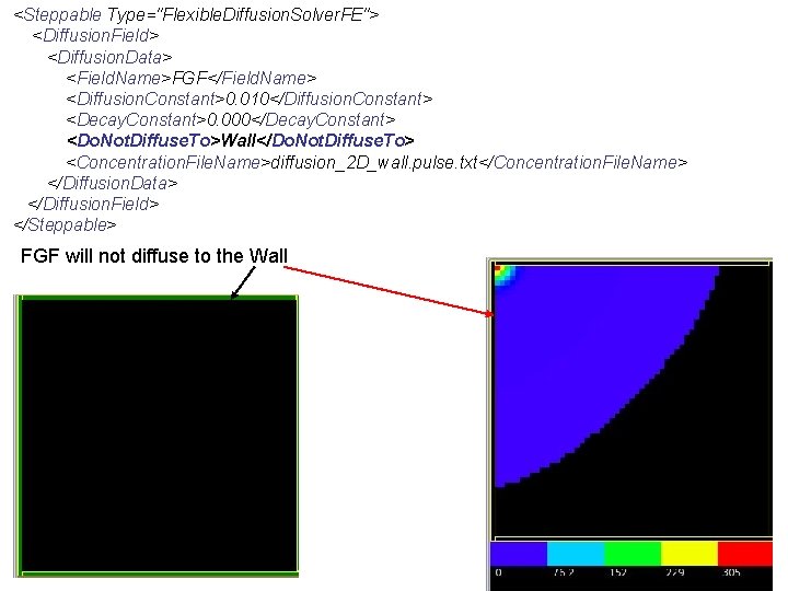
<Steppable Type="Flexible. Diffusion. Solver. FE"> <Diffusion. Field> <Diffusion. Data> <Field. Name>FGF</Field. Name> <Diffusion. Constant>0. 010</Diffusion. Constant> <Decay. Constant>0. 000</Decay. Constant> <Do. Not. Diffuse. To>Wall</Do. Not. Diffuse. To> <Concentration. File. Name>diffusion_2 D_wall. pulse. txt</Concentration. File. Name> </Diffusion. Data> </Diffusion. Field> </Steppable> FGF will not diffuse to the Wall

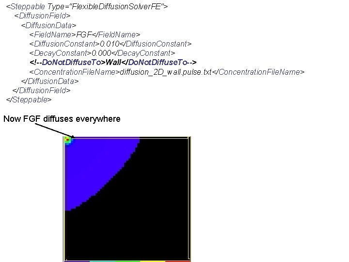
<Steppable Type="Flexible. Diffusion. Solver. FE"> <Diffusion. Field> <Diffusion. Data> <Field. Name>FGF</Field. Name> <Diffusion. Constant>0. 010</Diffusion. Constant> <Decay. Constant>0. 000</Decay. Constant> <!--Do. Not. Diffuse. To>Wall</Do. Not. Diffuse. To--> <Concentration. File. Name>diffusion_2 D_wall. pulse. txt</Concentration. File. Name> </Diffusion. Data> </Diffusion. Field> </Steppable> Now FGF diffuses everywhere

PDE Solver Caller Plugin By default PDE solver is called once per MCS. You may call it more often, say 3 times per MCS by including PDESolver. Caller plugin: <Plugin Name="PDESolver. Caller"> <Call. PDESolver. Name="Flexible. Diffusion. Solver. FE" Extra. Times. Per. MC=“ 2"/> </Plugin> Notice, that you may include multiple Call. PDE tags to call different PDESolvers with different frequencies. You typically use this plugin to avoid numerical instabilities when working with large diffusion constants

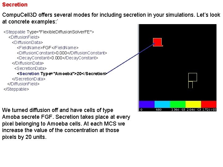
Secretion Compu. Cell 3 D offers several modes for including secretion in your simulations. Let’s look at concrete examples: ` <Steppable Type="Flexible. Diffusion. Solver. FE"> <Diffusion. Field> <Diffusion. Data> <Field. Name>FGF</Field. Name> <Diffusion. Constant>0. 000</Diffusion. Constant> <Decay. Constant>0. 000</Decay. Constant> </Diffusion. Data> <Secretion Type="Amoeba">20</Secretion> </Secretion. Data> </Diffusion. Field> </Steppable> We turned diffusion off and have cells of type Amoba secrete FGF. Secretion takes place at every pixel belonging to Amoeba cells. At each MCS we increase the value of the concentration at those pixels by 20 units.

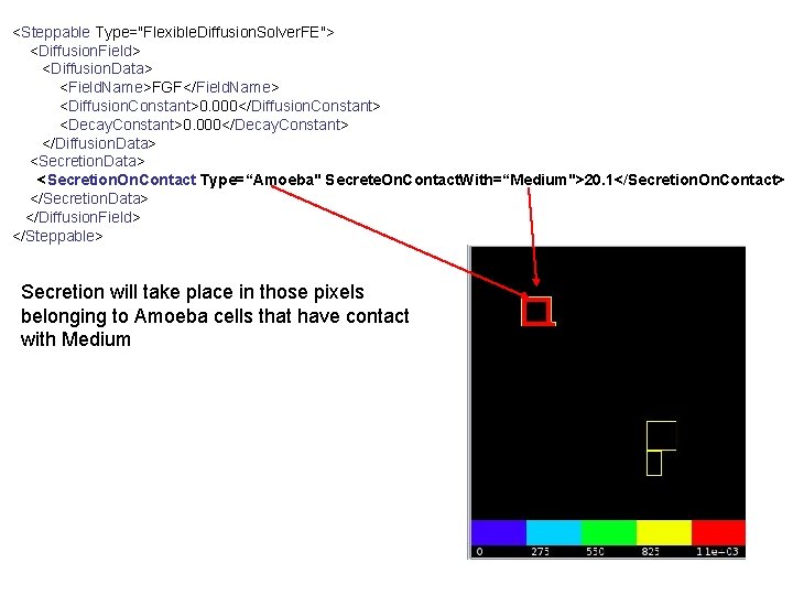
<Steppable Type="Flexible. Diffusion. Solver. FE"> <Diffusion. Field> <Diffusion. Data> <Field. Name>FGF</Field. Name> <Diffusion. Constant>0. 000</Diffusion. Constant> <Decay. Constant>0. 000</Decay. Constant> </Diffusion. Data> <Secretion. On. Contact Type=“Amoeba" Secrete. On. Contact. With=“Medium">20. 1</Secretion. On. Contact> </Secretion. Data> </Diffusion. Field> </Steppable> Secretion will take place in those pixels belonging to Amoeba cells that have contact with Medium

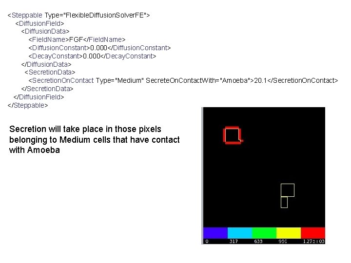
<Steppable Type="Flexible. Diffusion. Solver. FE"> <Diffusion. Field> <Diffusion. Data> <Field. Name>FGF</Field. Name> <Diffusion. Constant>0. 000</Diffusion. Constant> <Decay. Constant>0. 000</Decay. Constant> </Diffusion. Data> <Secretion. On. Contact Type="Medium" Secrete. On. Contact. With="Amoeba">20. 1</Secretion. On. Contact> </Secretion. Data> </Diffusion. Field> </Steppable> Secretion will take place in those pixels belonging to Medium cells that have contact with Amoeba

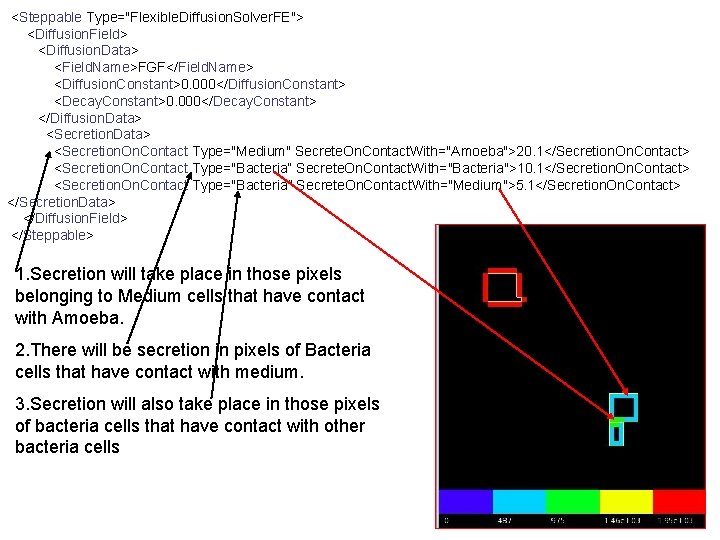
<Steppable Type="Flexible. Diffusion. Solver. FE"> <Diffusion. Field> <Diffusion. Data> <Field. Name>FGF</Field. Name> <Diffusion. Constant>0. 000</Diffusion. Constant> <Decay. Constant>0. 000</Decay. Constant> </Diffusion. Data> <Secretion. On. Contact Type="Medium" Secrete. On. Contact. With="Amoeba">20. 1</Secretion. On. Contact> <Secretion. On. Contact Type="Bacteria“ Secrete. On. Contact. With="Bacteria">10. 1</Secretion. On. Contact> <Secretion. On. Contact Type="Bacteria" Secrete. On. Contact. With="Medium">5. 1</Secretion. On. Contact> </Secretion. Data> </Diffusion. Field> </Steppable> 1. Secretion will take place in those pixels belonging to Medium cells that have contact with Amoeba. 2. There will be secretion in pixels of Bacteria cells that have contact with medium. 3. Secretion will also take place in those pixels of bacteria cells that have contact with other bacteria cells

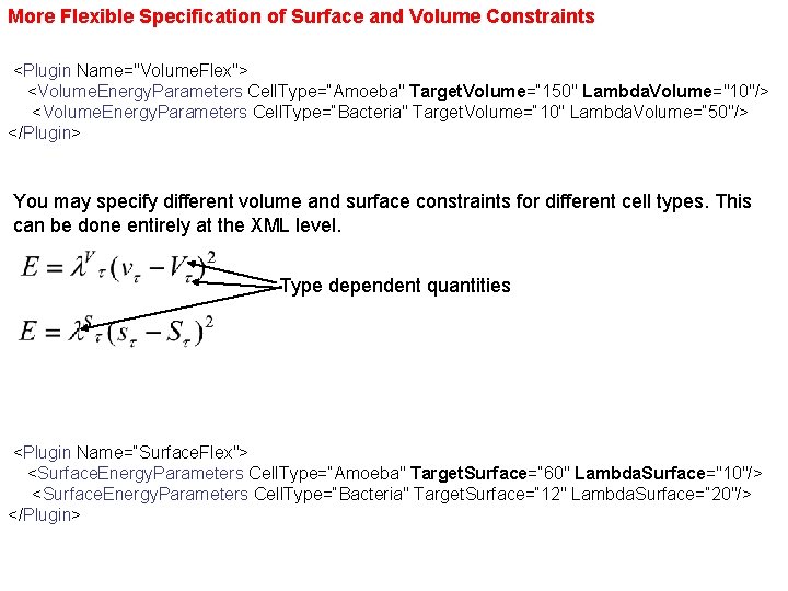
More Flexible Specification of Surface and Volume Constraints <Plugin Name="Volume. Flex"> <Volume. Energy. Parameters Cell. Type=“Amoeba" Target. Volume=“ 150" Lambda. Volume="10"/> <Volume. Energy. Parameters Cell. Type=“Bacteria" Target. Volume=“ 10" Lambda. Volume=“ 50"/> </Plugin> You may specify different volume and surface constraints for different cell types. This can be done entirely at the XML level. Type dependent quantities <Plugin Name=“Surface. Flex"> <Surface. Energy. Parameters Cell. Type=“Amoeba" Target. Surface=“ 60" Lambda. Surface="10"/> <Surface. Energy. Parameters Cell. Type=“Bacteria" Target. Surface=“ 12" Lambda. Surface=“ 20"/> </Plugin>

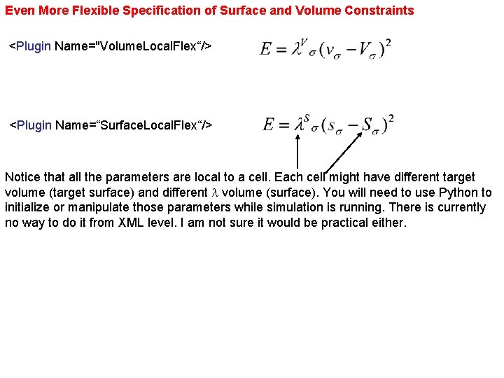
Even More Flexible Specification of Surface and Volume Constraints <Plugin Name="Volume. Local. Flex“/> <Plugin Name=“Surface. Local. Flex“/> Notice that all the parameters are local to a cell. Each cell might have different target volume (target surface) and different l volume (surface). You will need to use Python to initialize or manipulate those parameters while simulation is running. There is currently no way to do it from XML level. I am not sure it would be practical either.

Tracking Cell Neighbors Sometimes in your simulation you need to have access to a current list of cell neighbor. Compu. Cell 3 D makes this task easy: <Plugin Name=“Neighbor. Tracker“/> Inserting this statement in the plugins section of the XML will ensure that at any given time the list of cell neighbors will be accessible to the user. You can access such a list either using C++ or Python. In addition to storing neighbor list , a common surface area of a cell with its neighbors is stored.

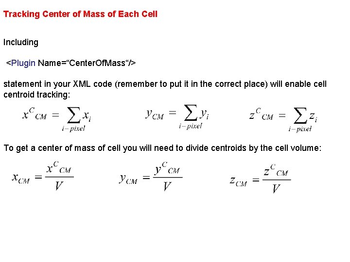
Tracking Center of Mass of Each Cell Including <Plugin Name=“Center. Of. Mass“/> statement in your XML code (remember to put it in the correct place) will enable cell centroid tracking: To get a center of mass of cell you will need to divide centroids by the cell volume:

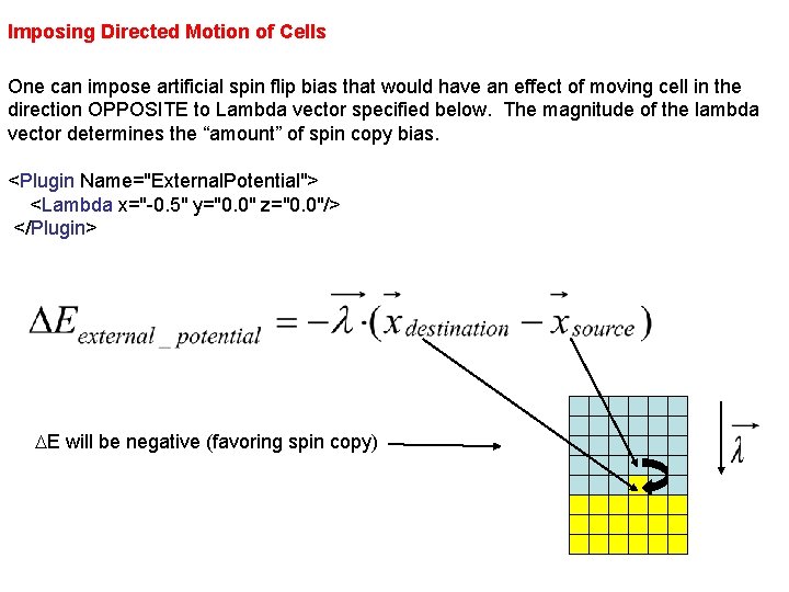
Imposing Directed Motion of Cells One can impose artificial spin flip bias that would have an effect of moving cell in the direction OPPOSITE to Lambda vector specified below. The magnitude of the lambda vector determines the “amount” of spin copy bias. <Plugin Name="External. Potential"> <Lambda x="-0. 5" y="0. 0" z="0. 0"/> </Plugin> DE will be negative (favoring spin copy)

Connectivity Plugin Connectivity plugin ensures that 2 D cells are not fragmented and are simply connected. It decreases probability of certain spin flips which are can break connectedness of a cell. Users can specify energy penalty that will be incured if the spin copy is to break connectedness of the cell. : Syntax: <Plugin Name=“Connectivity”> <Penalty>100000</Penalty> </Plugin>

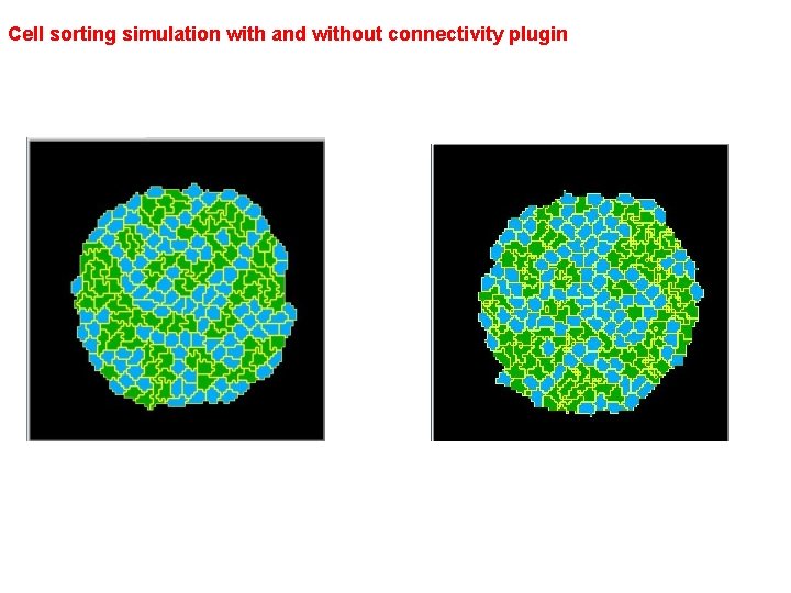
Cell sorting simulation with and without connectivity plugin

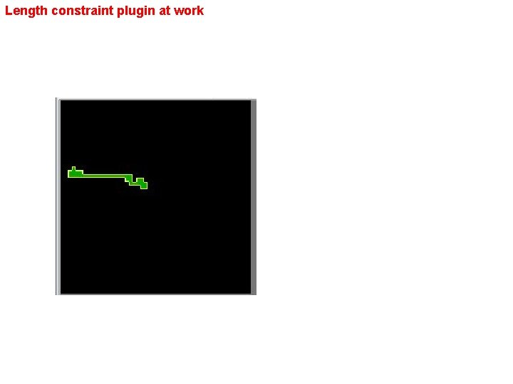
Length Constraint Plugin Length constraint plugin is used to force cells to keep preferred length along cell’s longest axis (we assume that cells have elliptical shape): <Plugin Name=“Length. Constraint”> <Length. Energy. Parameters Target. Length=“ 15” Lambda. Length=“ 2. 0”/> </Plugin> The Lambda. Length and Target. Length play similar role to Lambda. Volume and Target. Volume from Volume Plugin. IMPORTANT: Length Constraint Plugin has to be used together with connectivity plugin or else cells might become fragmented. The applicability of the Length. Constraint and Connectivity Plugins is limited to 2 D simulations. For more information see “Cell elongation is key to in silico replication of in vitro vasculogenesis and subsequent remodeling” by Roeland M. H. Merks et al Developmental Biology 289 (2006) 44– 54

Length constraint plugin at work

scripting inside Compu. Cell 3 D XML gives you the ability to change simulation parameters using human-readable syntax but does not allow users to implement more complex cell behaviors, sophisticated cell type transition rules, inter-cell signaling or connecting to intracellular models Python scripting capabilities in Compu. Cell 3 D allow users to accomplish abovementioned tasks (and much more) and are the reasons why Compu. Cell 3 D is called simulation environment, not simulation application. Python scripting capabilities allow users to use rich set of Python modules and third party libraries and provide level flexibility comparable with packages such as Matlab or Mathematica

Python Scripting Prerequisites • To make full use of Python scripting users should be familiar with Python programming language. They do not need to be experts though. • Compu. Cell 3 D comes with template and example codes that make Python scripting inside Compu. Cell 3 D quite easy even for beginners. • Python scripting in Compu. Cell 3 D typically requires users to develop a class that implements required logic. If you are unfamiliar with concept of class , think of it as a type that has several data members (such as floats, integers, other classes) and set of functions that operate on those internal members but can also take external arguments. Class is a generalization of “C” structure or “Pascal” record. • Fortunately Compu. Cell 3 D comes with plenty of examples that users can adapt to serve their needs. This does not require thorough programming knowledge. If you are unfamiliar with Python scripting, reading (and doing) “Compu. Cell 3 D Python Scripting Tutorials” should quickly get you up-to-speed.

Where Do You Begin? • You will still need XML file describing which plugins and/or steppables Compu. Cell 3 D is to use. In the future releases we might change this requirement but for now it appeared as the best way of ensuring proper module initialization • In addition to XML file you will need to write Python script that implements main Compu. Cell 3 D logic i. e. reads XML file, initializes modules and executes calls in a loop Metropolis algorithm. This file will also call set up and initialize your modules written in Python. Compu. Cell 3 D comes with many examples of such files so in fact preparing one is reduced to minor modification of existing one. • Once you have XML and Python scripts ready you opent them up in the Player and start running simulaitons

What Can You Do in Python? You may implement any Compu. Cell 3 D module using Python – energy functions, lattice monitors, steppers, steppables, fixed steppers. You need to remember that Python is an interpreted language and thus executes orders of magnitudes slower than for example C++. This means that although you can easily develop energy functions (remember, they are the most frequently called modules in Compu. Cell 3 D) in Python, you will probably want to avoid using them with your “production runs”. In this it makes sense to implement those functions in C++ , which is not too difficult and we provide comprehensive Developers documentation. Since lattice monitors are called less frequently than energy functions, the performance degradation due to lattice monitor being implemented in Python is much smaller. That same is true for steppers, fixed steppers and steppables. Notice that Compu. Cell 3 D kernel that is called from Python, as well as other core Compu. Cell 3 D modules called from Python run at native speeds, as they are implemented in C++ with only their API exposed to Python. Therefore if you run Compu. Cell 3 D through Python script but decide not to implement new Python modules, your speed of run will be essentially identical as if you ran Compu. Cell 3 D using just XML file.

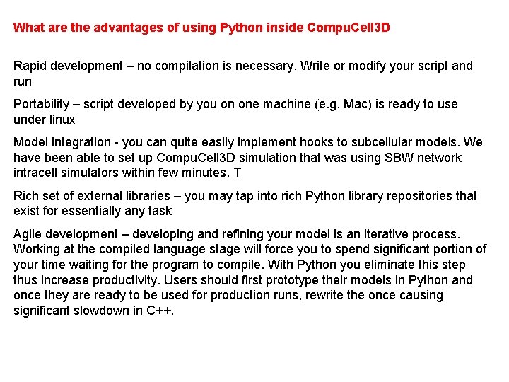
What are the advantages of using Python inside Compu. Cell 3 D Rapid development – no compilation is necessary. Write or modify your script and run Portability – script developed by you on one machine (e. g. Mac) is ready to use under linux Model integration - you can quite easily implement hooks to subcellular models. We have been able to set up Compu. Cell 3 D simulation that was using SBW network intracell simulators within few minutes. T Rich set of external libraries – you may tap into rich Python library repositories that exist for essentially any task Agile development – developing and refining your model is an iterative process. Working at the compiled language stage will force you to spend significant portion of your time waiting for the program to compile. With Python you eliminate this step thus increase productivity. Users should first prototype their models in Python and once they are ready to be used for production runs, rewrite the once causing significant slowdown in C++.

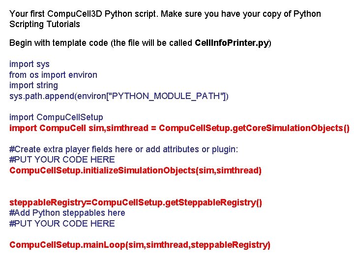
Your first Compu. Cell 3 D Python script. Make sure you have your copy of Python Scripting Tutorials Begin with template code (the file will be called Cell. Info. Printer. py) import sys from os import environ import string sys. path. append(environ["PYTHON_MODULE_PATH"]) import Compu. Cell. Setup import Compu. Cell sim, simthread = Compu. Cell. Setup. get. Core. Simulation. Objects() #Create extra player fields here or add attributes or plugin: #PUT YOUR CODE HERE Compu. Cell. Setup. initialize. Simulation. Objects(sim, simthread) steppable. Registry=Compu. Cell. Setup. get. Steppable. Registry() #Add Python steppables here #PUT YOUR CODE HERE Compu. Cell. Setup. main. Loop(sim, simthread, steppable. Registry)

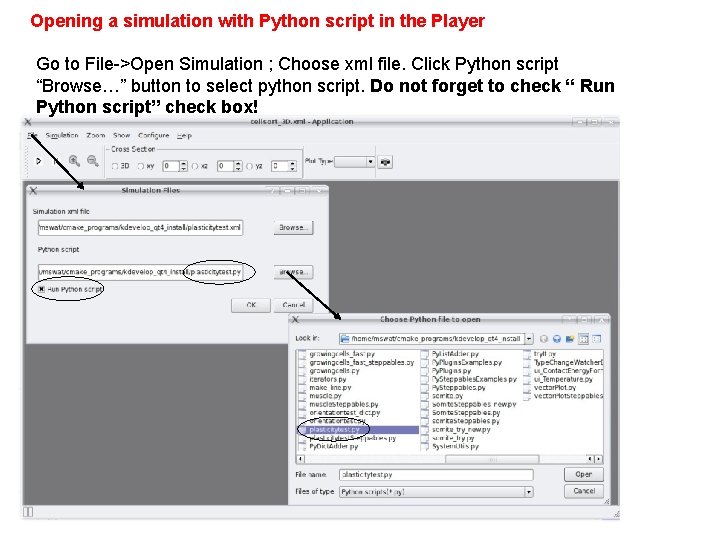
Opening a simulation with Python script in the Player Go to File->Open Simulation ; Choose xml file. Click Python script “Browse…” button to select python script. Do not forget to check “ Run Python script” check box!

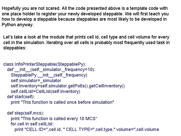
Hopefully you are not scared. All the code presented above is a template code with one place holder to register your newly developed steppable. We will first teach you how to develop a steppable because steppables are most likely to be developed in Python anyway. Let’s take a look at the module that prints cell id, cell type and cell volume for every cell in the simulation. Iterating over all cells is probably most frequently used task in steppables: class Info. Printer. Steppable(Steppable. Py): def __init__(self, _simulator, _frequency=10): Steppable. Py. __init__(self, _frequency) self. simulator=_simulator self. inventory=self. simulator. get. Potts(). get. Cell. Inventory() self. cell. List=Cell. List(self. inventory) def start(self): print "This function is called once before simulation" def step(self, mcs): print "This function is called every 10 MCS“ for cell in self. cell. List: print "CELL ID=", cell. id, " CELL TYPE=", cell. type, " volume=", cell. volume

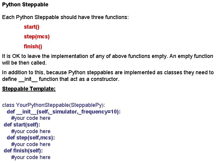
Python Steppable Each Python Steppable should have three functions: start() step(mcs) finish() It is OK to leave the implementation of any of above functions empty. An empty function will be then called. In addition to this, because Python steppables are implemented as classes they need to define __init__ function that act as a constructor. Steppable Template: class Your. Python. Steppable(Steppable. Py): def __init__(self, _simulator, _frequency=10): #your code here def start(self): #your code here def step(self, mcs): #your code here def finish(self): #your code here

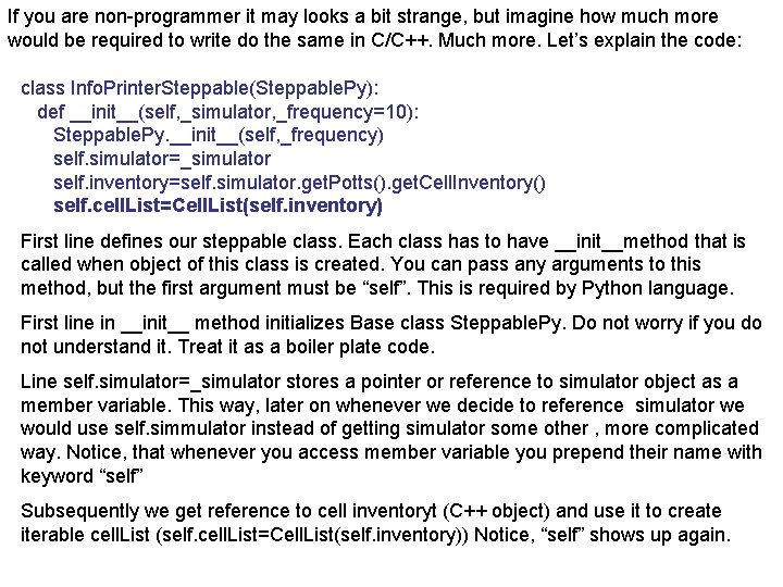
If you are non-programmer it may looks a bit strange, but imagine how much more would be required to write do the same in C/C++. Much more. Let’s explain the code: class Info. Printer. Steppable(Steppable. Py): def __init__(self, _simulator, _frequency=10): Steppable. Py. __init__(self, _frequency) self. simulator=_simulator self. inventory=self. simulator. get. Potts(). get. Cell. Inventory() self. cell. List=Cell. List(self. inventory) First line defines our steppable class. Each class has to have __init__method that is called when object of this class is created. You can pass any arguments to this method, but the first argument must be “self”. This is required by Python language. First line in __init__ method initializes Base class Steppable. Py. Do not worry if you do not understand it. Treat it as a boiler plate code. Line self. simulator=_simulator stores a pointer or reference to simulator object as a member variable. This way, later on whenever we decide to reference simulator we would use self. simmulator instead of getting simulator some other , more complicated way. Notice, that whenever you access member variable you prepend their name with keyword “self” Subsequently we get reference to cell inventoryt (C++ object) and use it to create iterable cell. List (self. cell. List=Cell. List(self. inventory)) Notice, “self” shows up again.

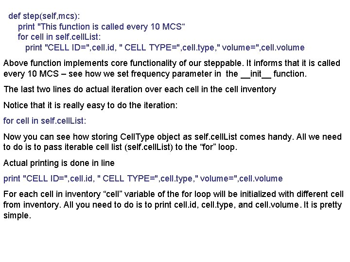
def step(self, mcs): print "This function is called every 10 MCS“ for cell in self. cell. List: print "CELL ID=", cell. id, " CELL TYPE=", cell. type, " volume=", cell. volume Above function implements core functionality of our steppable. It informs that it is called every 10 MCS – see how we set frequency parameter in the __init__ function. The last two lines do actual iteration over each cell in the cell inventory Notice that it is really easy to do the iteration: for cell in self. cell. List: Now you can see how storing Cell. Type object as self. cell. List comes handy. All we need to do is to pass iterable cell list (self. cell. List) to the “for” loop. Actual printing is done in line print "CELL ID=", cell. id, " CELL TYPE=", cell. type, " volume=", cell. volume For each cell in inventory “cell” variable of the for loop will be initialized with different cell from inventory. All you need to do is to print cell. id, cell. type, and cell. volume. It is pretty simple.

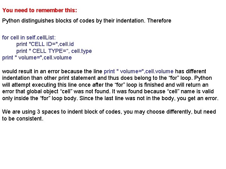
You need to remember this: Python distinguishes blocks of codes by their indentation. Therefore for cell in self. cell. List: print "CELL ID=", cell. id print " CELL TYPE=“, cell. type print " volume=", cell. volume would result in an error because the line print " volume=", cell. volume has different indentation than other print statement and thus does belong to the “for” loop. Python will attempt executing this line once after the “for” loop is finished and will return an error that global object “cell” was not found. It was found because “cell” name is valid only inside the “for” loop body. Since the last line was not in the body, you get an error. We are using 3 spaces to indent block of codes, you may choose differently, but need to be consistent.

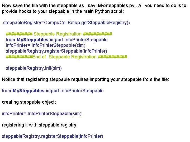
Now save the file with the steppable as , say, My. Steppables. py. All you need to do is to provide hooks to your steppable in the main Python script: steppable. Registry=Compu. Cell. Setup. get. Steppable. Registry() ##### Steppable Registration ###### from My. Steppables import Info. Printer. Steppable info. Printer= Info. Printer. Steppable(sim) steppable. Registry. register. Steppable(info. Printer) #####End of Steppable Registration ###### steppable. Registry. init(sim) Notice that registering steppable requires importing your steppable from the file: from My. Steppables import Info. Printer. Steppable creating steppable object: info. Printer= Info. Printer. Steppable(sim) registering it with steppable registry: steppable. Registry. register. Steppable(info. Printer)

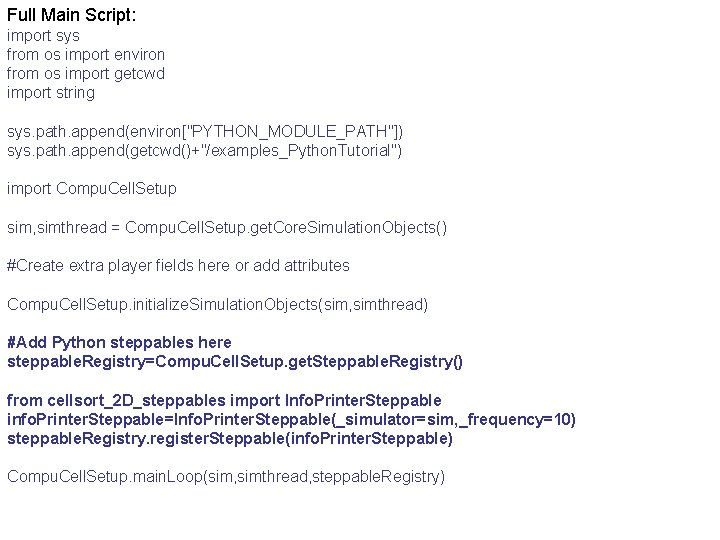
Full Main Script: import sys from os import environ from os import getcwd import string sys. path. append(environ["PYTHON_MODULE_PATH"]) sys. path. append(getcwd()+"/examples_Python. Tutorial") import Compu. Cell. Setup sim, simthread = Compu. Cell. Setup. get. Core. Simulation. Objects() #Create extra player fields here or add attributes Compu. Cell. Setup. initialize. Simulation. Objects(sim, simthread) #Add Python steppables here steppable. Registry=Compu. Cell. Setup. get. Steppable. Registry() from cellsort_2 D_steppables import Info. Printer. Steppable info. Printer. Steppable=Info. Printer. Steppable(_simulator=sim, _frequency=10) steppable. Registry. register. Steppable(info. Printer. Steppable) Compu. Cell. Setup. main. Loop(sim, simthread, steppable. Registry)

Now, all you need to do is to open in the Player previous xml file (cellsort_2 D. xml) together with newly created Cell. Info. Printer. py and check Run Python check box. Notice that you are not loading directly My. Stappables. py file. The module you stored to this file will be called from Cell. Info. Printer. py. Try running the simulation and see if you got any performance degradation. Probably not, but by using Python you have saved yourself a lot of tedious C++ coding, not to mention that you do not need to care about dependencies, compilation, etc. . Writing your next Python steppable will require much less effort as well, as you will quickly discover that you will be using same basic code template all over again. Instead of thinking how the code you are writing fits in the overall framework you will just concentrate on it’s core functionality and leave the rest to Compu. Cell 3 D. In case you wonder how this is all possible , it is due to Object Oriented programming. Hopefully this short tutorial will encourage you to learn more of object oriented programming. It is really worth the effort.

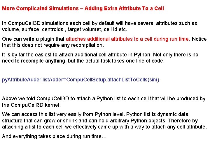
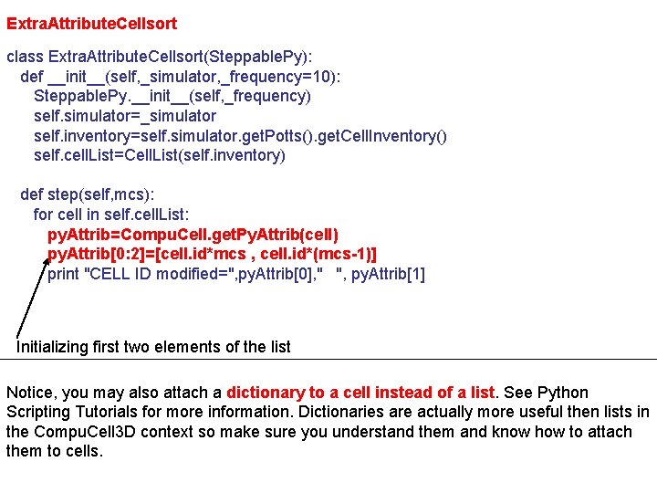
More Complicated Simulations – Adding Extra Attribute To a Cell In Compu. Cell 3 D simulations each cell by default will have several attributes such as volume, surface, centroids , target volumet, cell id etc. One can write a plugin that attaches additional attributes to a cell during run time. Notice that this does not require any recompilation. It is by far the easiest to attach additional cell attribute in Python. Not only there is no need to recompile anything, but the actual task takes one line of code: py. Attribute. Adder, list. Adder=Compu. Cell. Setup. attach. List. To. Cells(sim) Above we told Compu. Cell 3 D to attach a Python list to each cell that will be produced by the Compu. Cell 3 D kernel. We can access this list very easily from Python level. Python list is dynamic data structure that can grow or shrink and can hold arbitrary Python objects. Therefore by attaching a list to each cell we effectively came up with a way to attach any cell attribute. And everything takes place during run time…

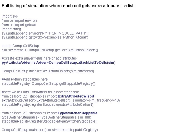
Full listing of simulation where each cell gets extra attribute – a list: import sys from os import environ from os import getcwd import string sys. path. append(environ["PYTHON_MODULE_PATH"]) sys. path. append(getcwd()+"/examples_Python. Tutorial") import Compu. Cell. Setup sim, simthread = Compu. Cell. Setup. get. Core. Simulation. Objects() #Create extra player fields here or add attributes py. Attribute. Adder, list. Adder=Compu. Cell. Setup. attach. List. To. Cells(sim) Compu. Cell. Setup. initialize. Simulation. Objects(sim, simthread) #Add Python steppables here steppable. Registry=Compu. Cell. Setup. get. Steppable. Registry() #here we will add Extra. Attribute. Cellsort steppable from cellsort_2 D_steppables import Extra. Attribute. Cellsort extra. Attribute. Cellsort=Extra. Attribute. Cellsort(_simulator=sim, _frequency=10) steppable. Registry. register. Steppable(extra. Attribute. Cellsort) from cellsort_2 D_steppables import Type. Switcher. Steppable type. Switcher. Steppable=Type. Switcher. Steppable(sim, 100) steppable. Registry. register. Steppable(type. Switcher. Steppable) Compu. Cell. Setup. main. Loop(sim, simthread, steppable. Registry)

Extra. Attribute. Cellsort class Extra. Attribute. Cellsort(Steppable. Py): def __init__(self, _simulator, _frequency=10): Steppable. Py. __init__(self, _frequency) self. simulator=_simulator self. inventory=self. simulator. get. Potts(). get. Cell. Inventory() self. cell. List=Cell. List(self. inventory) def step(self, mcs): for cell in self. cell. List: py. Attrib=Compu. Cell. get. Py. Attrib(cell) py. Attrib[0: 2]=[cell. id*mcs , cell. id*(mcs-1)] print "CELL ID modified=", py. Attrib[0], " ", py. Attrib[1] Initializing first two elements of the list Notice, you may also attach a dictionary to a cell instead of a list. See Python Scripting Tutorials for more information. Dictionaries are actually more useful then lists in the Compu. Cell 3 D context so make sure you understand them and know how to attach them to cells.

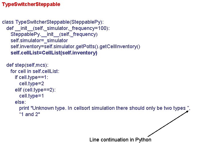
Type. Switcher. Steppable class Type. Switcher. Steppable(Steppable. Py): def __init__(self, _simulator, _frequency=100): Steppable. Py. __init__(self, _frequency) self. simulator=_simulator self. inventory=self. simulator. get. Potts(). get. Cell. Inventory() self. cell. List=Cell. List(self. inventory) def step(self, mcs): for cell in self. cell. List: if cell. type==1: cell. type=2 elif (cell. type==2): cell. type=1 else: print "Unknown type. In cellsort simulation there should only be two types ”, “ 1 and 2" Line continuation in Python

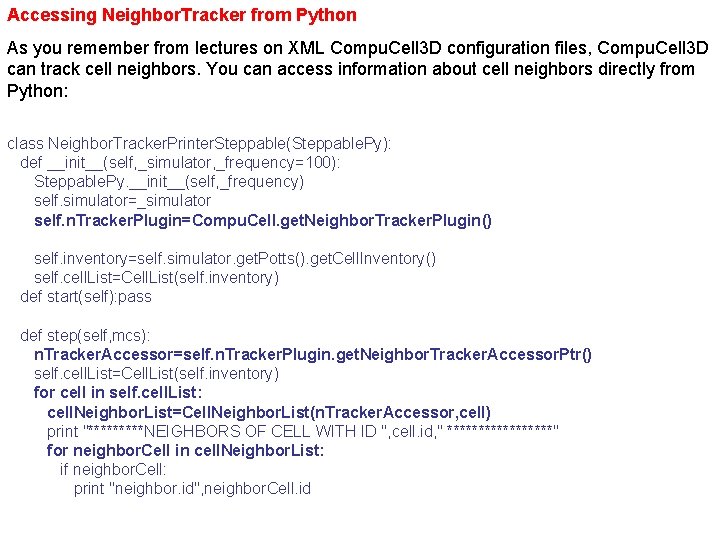
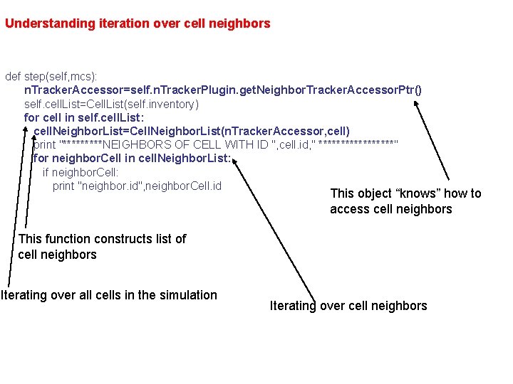
Accessing Neighbor. Tracker from Python As you remember from lectures on XML Compu. Cell 3 D configuration files, Compu. Cell 3 D can track cell neighbors. You can access information about cell neighbors directly from Python: class Neighbor. Tracker. Printer. Steppable(Steppable. Py): def __init__(self, _simulator, _frequency=100): Steppable. Py. __init__(self, _frequency) self. simulator=_simulator self. n. Tracker. Plugin=Compu. Cell. get. Neighbor. Tracker. Plugin() self. inventory=self. simulator. get. Potts(). get. Cell. Inventory() self. cell. List=Cell. List(self. inventory) def start(self): pass def step(self, mcs): n. Tracker. Accessor=self. n. Tracker. Plugin. get. Neighbor. Tracker. Accessor. Ptr() self. cell. List=Cell. List(self. inventory) for cell in self. cell. List: cell. Neighbor. List=Cell. Neighbor. List(n. Tracker. Accessor, cell) print "*****NEIGHBORS OF CELL WITH ID ", cell. id, " *********" for neighbor. Cell in cell. Neighbor. List: if neighbor. Cell: print "neighbor. id", neighbor. Cell. id

Understanding iteration over cell neighbors def step(self, mcs): n. Tracker. Accessor=self. n. Tracker. Plugin. get. Neighbor. Tracker. Accessor. Ptr() self. cell. List=Cell. List(self. inventory) for cell in self. cell. List: cell. Neighbor. List=Cell. Neighbor. List(n. Tracker. Accessor, cell) print "*****NEIGHBORS OF CELL WITH ID ", cell. id, " *********" for neighbor. Cell in cell. Neighbor. List: if neighbor. Cell: print "neighbor. id", neighbor. Cell. id This object “knows” how to access cell neighbors This function constructs list of cell neighbors Iterating over all cells in the simulation Iterating over cell neighbors

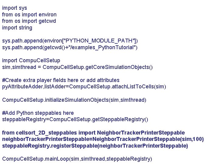
import sys from os import environ from os import getcwd import string sys. path. append(environ["PYTHON_MODULE_PATH"]) sys. path. append(getcwd()+"/examples_Python. Tutorial") import Compu. Cell. Setup sim, simthread = Compu. Cell. Setup. get. Core. Simulation. Objects() #Create extra player fields here or add attributes py. Attribute. Adder, list. Adder=Compu. Cell. Setup. attach. List. To. Cells(sim) Compu. Cell. Setup. initialize. Simulation. Objects(sim, simthread) #Add Python steppables here steppable. Registry=Compu. Cell. Setup. get. Steppable. Registry() from cellsort_2 D_steppables import Neighbor. Tracker. Printer. Steppable neighbor. Tracker. Printer. Steppable=Neighbor. Tracker. Printer. Steppable(sim, 100) steppable. Registry. register. Steppable(neighbor. Tracker. Printer. Steppable) Compu. Cell. Setup. main. Loop(sim, simthread, steppable. Registry)

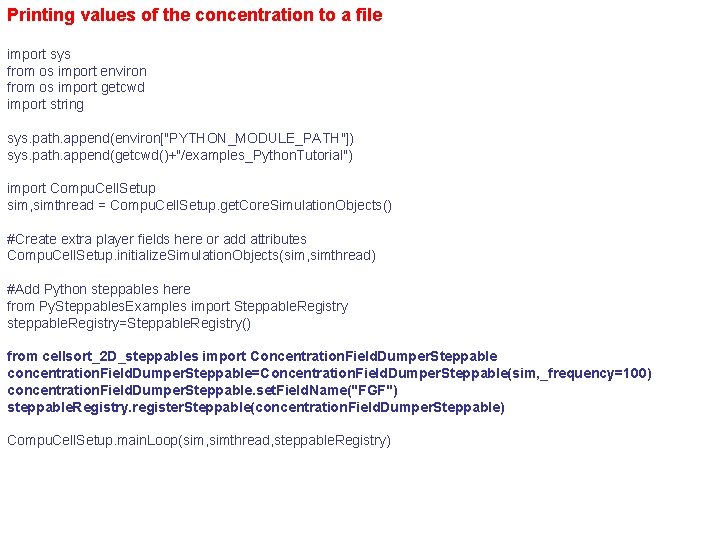
Printing values of the concentration to a file import sys from os import environ from os import getcwd import string sys. path. append(environ["PYTHON_MODULE_PATH"]) sys. path. append(getcwd()+"/examples_Python. Tutorial") import Compu. Cell. Setup sim, simthread = Compu. Cell. Setup. get. Core. Simulation. Objects() #Create extra player fields here or add attributes Compu. Cell. Setup. initialize. Simulation. Objects(sim, simthread) #Add Python steppables here from Py. Steppables. Examples import Steppable. Registry steppable. Registry=Steppable. Registry() from cellsort_2 D_steppables import Concentration. Field. Dumper. Steppable concentration. Field. Dumper. Steppable=Concentration. Field. Dumper. Steppable(sim, _frequency=100) concentration. Field. Dumper. Steppable. set. Field. Name("FGF") steppable. Registry. register. Steppable(concentration. Field. Dumper. Steppable) Compu. Cell. Setup. main. Loop(sim, simthread, steppable. Registry)

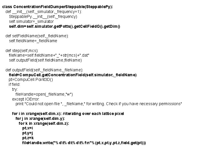
class Concentration. Field. Dumper. Steppable(Steppable. Py): def __init__(self, _simulator, _frequency=1): Steppable. Py. __init__(self, _frequency) self. simulator=_simulator self. dim=self. simulator. get. Potts(). get. Cell. Field. G(). get. Dim() def set. Field. Name(self, _field. Name): self. field. Name=_field. Name def step(self, mcs): file. Name=self. field. Name+"_"+str(mcs)+". dat" self. output. Field(self. field. Name, file. Name) def output. Field(self, _field. Name, _file. Name): field=Compu. Cell. get. Concentration. Field(self. simulator, _field. Name) pt=Compu. Cell. Point 3 D() if field: try: file. Handle=open(_file. Name, "w") except IOError: print "Could not open file ", _file. Name, " for writing. Check if you have necessary permissions" for i in xrange(self. dim. x): #iterating over each lattice pixel for j in xrange(self. dim. y): for k in xrange(self. dim. z): pt. x=i pt. y=j pt. z=k file. Handle. write("%dt%dt%fn"%(pt. x, pt. y, pt. z, field. get(pt)))

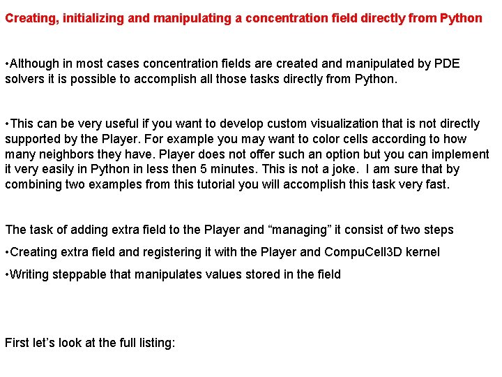
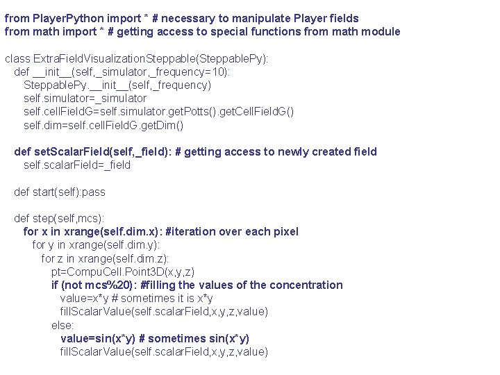
Creating, initializing and manipulating a concentration field directly from Python • Although in most cases concentration fields are created and manipulated by PDE solvers it is possible to accomplish all those tasks directly from Python. • This can be very useful if you want to develop custom visualization that is not directly supported by the Player. For example you may want to color cells according to how many neighbors they have. Player does not offer such an option but you can implement it very easily in Python in less then 5 minutes. This is not a joke. I am sure that by combining two examples from this tutorial you will accomplish this task very fast. The task of adding extra field to the Player and “managing” it consist of two steps • Creating extra field and registering it with the Player and Compu. Cell 3 D kernel • Writing steppable that manipulates values stored in the field First let’s look at the full listing:

from os import environ from os import getcwd import string sys. path. append(environ["PYTHON_MODULE_PATH"]) sys. path. append(getcwd()+"/examples_Python. Tutorial") import Compu. Cell. Setup sim, simthread = Compu. Cell. Setup. get. Core. Simulation. Objects() import Compu. Cell Creating extra field is is really easy. The location of the function call that creates the field is , however important. See the comment #Create extra player fields here or add attributes dim=sim. get. Potts(). get. Cell. Field. G(). get. Dim() extra. Player. Field=simthread. create. Float. Field. Py(dim, "Extra. Field") Compu. Cell. Setup. initialize. Simulation. Objects(sim, simthread) #Add Python steppables here from Py. Steppables. Examples import Steppable. Registry steppable. Registry=Steppable. Registry() from cellsort_2 D_steppables import Extra. Field. Visualization. Steppable extra. Field. Visualization. Steppable=Extra. Field. Visualization. Steppable(_simulator=sim, _frequency=10) extra. Field. Visualization. Steppable. set. Scalar. Field(extra. Player. Field) steppable. Registry. register. Steppable(extra. Field. Visualization. Steppable) Compu. Cell. Setup. main. Loop(sim, simthread, steppable. Registry)

from Player. Python import * # necessary to manipulate Player fields from math import * # getting access to special functions from math module class Extra. Field. Visualization. Steppable(Steppable. Py): def __init__(self, _simulator, _frequency=10): Steppable. Py. __init__(self, _frequency) self. simulator=_simulator self. cell. Field. G=self. simulator. get. Potts(). get. Cell. Field. G() self. dim=self. cell. Field. G. get. Dim() def set. Scalar. Field(self, _field): # getting access to newly created field self. scalar. Field=_field def start(self): pass def step(self, mcs): for x in xrange(self. dim. x): #iteration over each pixel for y in xrange(self. dim. y): for z in xrange(self. dim. z): pt=Compu. Cell. Point 3 D(x, y, z) if (not mcs%20): #filling the values of the concentration value=x*y # sometimes it is x*y fill. Scalar. Value(self. scalar. Field, x, y, z, value) else: value=sin(x*y) # sometimes sin(x*y) fill. Scalar. Value(self. scalar. Field, x, y, z, value)

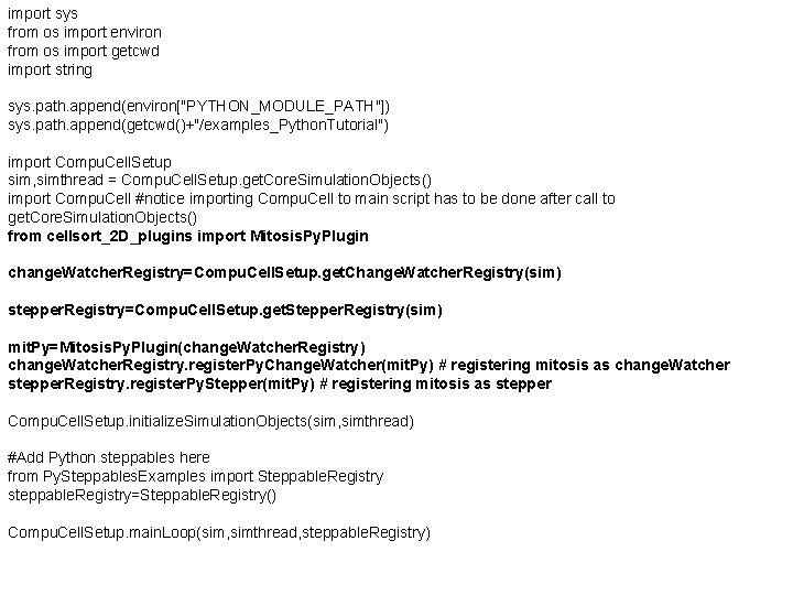
Mitosis in Compu. Cell 3 D simulations Supporting cell division (mitosis) in Compu. Cell 3 D simulations is a prerequisite for building faithful biomedical simulations. You can use mitosis module (Mitosis Plugin) directly from XML however, its use will be very limited because of the following fact: After cell division you end up with two cells. What parameters should those two cells have (type, target volume etc. )? How do you modify the parameters? The best solution is to manage mitosis from Python and the example below will explain you how to do it.

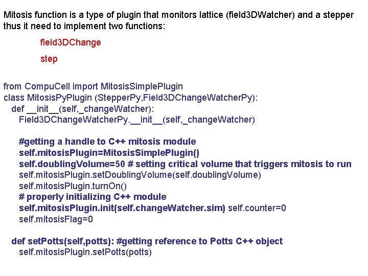
import sys from os import environ from os import getcwd import string sys. path. append(environ["PYTHON_MODULE_PATH"]) sys. path. append(getcwd()+"/examples_Python. Tutorial") import Compu. Cell. Setup sim, simthread = Compu. Cell. Setup. get. Core. Simulation. Objects() import Compu. Cell #notice importing Compu. Cell to main script has to be done after call to get. Core. Simulation. Objects() from cellsort_2 D_plugins import Mitosis. Py. Plugin change. Watcher. Registry=Compu. Cell. Setup. get. Change. Watcher. Registry(sim) stepper. Registry=Compu. Cell. Setup. get. Stepper. Registry(sim) mit. Py=Mitosis. Py. Plugin(change. Watcher. Registry) change. Watcher. Registry. register. Py. Change. Watcher(mit. Py) # registering mitosis as change. Watcher stepper. Registry. register. Py. Stepper(mit. Py) # registering mitosis as stepper Compu. Cell. Setup. initialize. Simulation. Objects(sim, simthread) #Add Python steppables here from Py. Steppables. Examples import Steppable. Registry steppable. Registry=Steppable. Registry() Compu. Cell. Setup. main. Loop(sim, simthread, steppable. Registry)

Mitosis function is a type of plugin that monitors lattice (field 3 DWatcher) and a stepper thus it need to implement two functions: field 3 DChange step from Compu. Cell import Mitosis. Simple. Plugin class Mitosis. Py. Plugin (Stepper. Py, Field 3 DChange. Watcher. Py): def __init__(self, _change. Watcher): Field 3 DChange. Watcher. Py. __init__(self, _change. Watcher) #getting a handle to C++ mitosis module self. mitosis. Plugin=Mitosis. Simple. Plugin() self. doubling. Volume=50 # setting critical volume that triggers mitosis to run self. mitosis. Plugin. set. Doubling. Volume(self. doubling. Volume) self. mitosis. Plugin. turn. On() # properly initializing C++ module self. mitosis. Plugin. init(self. change. Watcher. sim) self. counter=0 self. mitosis. Flag=0 def set. Potts(self, potts): #getting reference to Potts C++ object self. mitosis. Plugin. set. Potts(potts)

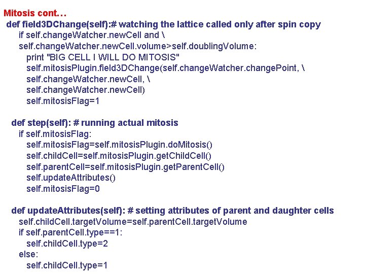
Mitosis cont… def field 3 DChange(self): # watching the lattice called only after spin copy if self. change. Watcher. new. Cell and self. change. Watcher. new. Cell. volume>self. doubling. Volume: print "BIG CELL I WILL DO MITOSIS" self. mitosis. Plugin. field 3 DChange(self. change. Watcher. change. Point, self. change. Watcher. new. Cell) self. mitosis. Flag=1 def step(self): # running actual mitosis if self. mitosis. Flag: self. mitosis. Flag=self. mitosis. Plugin. do. Mitosis() self. child. Cell=self. mitosis. Plugin. get. Child. Cell() self. parent. Cell=self. mitosis. Plugin. get. Parent. Cell() self. update. Attributes() self. mitosis. Flag=0 def update. Attributes(self): # setting attributes of parent and daughter cells self. child. Cell. target. Volume=self. parent. Cell. target. Volume if self. parent. Cell. type==1: self. child. Cell. type=2 else: self. child. Cell. type=1

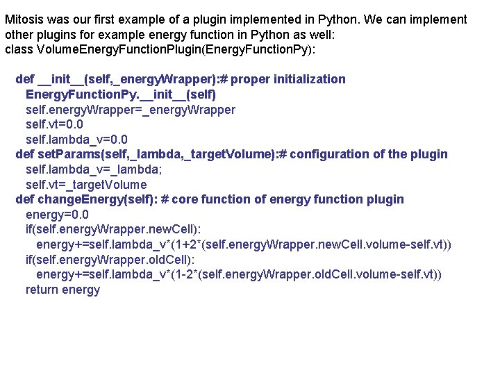
Mitosis was our first example of a plugin implemented in Python. We can implement other plugins for example energy function in Python as well: class Volume. Energy. Function. Plugin(Energy. Function. Py): def __init__(self, _energy. Wrapper): # proper initialization Energy. Function. Py. __init__(self) self. energy. Wrapper=_energy. Wrapper self. vt=0. 0 self. lambda_v=0. 0 def set. Params(self, _lambda, _target. Volume): # configuration of the plugin self. lambda_v=_lambda; self. vt=_target. Volume def change. Energy(self): # core function of energy function plugin energy=0. 0 if(self. energy. Wrapper. new. Cell): energy+=self. lambda_v*(1+2*(self. energy. Wrapper. new. Cell. volume-self. vt)) if(self. energy. Wrapper. old. Cell): energy+=self. lambda_v*(1 -2*(self. energy. Wrapper. old. Cell. volume-self. vt)) return energy

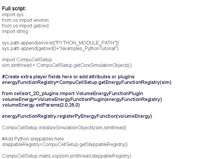
Full script: import sys from os import environ from os import getcwd import string sys. path. append(environ["PYTHON_MODULE_PATH"]) sys. path. append(getcwd()+"/examples_Python. Tutorial") import Compu. Cell. Setup sim, simthread = Compu. Cell. Setup. get. Core. Simulation. Objects() #Create extra player fields here or add attributes or plugins energy. Function. Registry=Compu. Cell. Setup. get. Energy. Function. Registry(sim) from cellsort_2 D_plugins import Volume. Energy. Function. Plugin volume. Energy=Volume. Energy. Function. Plugin(energy. Function. Registry) volume. Energy. set. Params(2. 0, 25. 0) energy. Function. Registry. register. Py. Energy. Function(volume. Energy) Compu. Cell. Setup. initialize. Simulation. Objects(sim, simthread) #Add Python steppables here steppable. Registry=Compu. Cell. Setup. get. Steppable. Registry() Compu. Cell. Setup. main. Loop(sim, simthread, steppable. Registry)

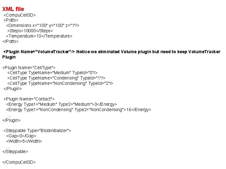
XML file <Compu. Cell 3 D> <Potts> <Dimensions x="100" y="100" z="1"/> <Steps>10000</Steps> <Temperature>10</Temperature> </Potts> <Plugin Name="Volume. Tracker"/> Notice we eliminated Volume plugin but need to keep Volume. Tracker Plugin <Plugin Name="Cell. Type"> <Cell. Type. Name="Medium" Type. Id="0"/> <Cell. Type. Name="Condensing" Type. Id="1"/> <Cell. Type. Name="Non. Condensing" Type. Id="2"/> </Plugin> <Plugin Name="Contact"> <Energy Type 1="Medium" Type 2="Medium">0</Energy> <Energy Type 1="Non. Condensing" Type 2="Non. Condensing">16</Energy> … </Plugin> <Steppable Type="Blob. Initializer"> <Gap>0</Gap> <Width>5</Width> … </Steppable> </Compu. Cell 3 D>

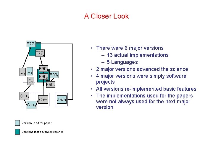
Why Compu. Cell 3 D and why now? Typical Evolution of Research Software (in collaboration with Chris Mueller) • First application written in Fortran F 77 C • Tom ports to C • Adds command line parameters, makefile • Jenny ports to F 90 • Extends model F 90 • Brad ports to C++ • Models system using objects C++ Java • Maria implements simulation in Java for the Grid • Implements original model • Sounds familiar? Keep listening…

A Closer Look F 771 F 772 C 1 C 3 C 2 C++1 F 903 F 902 F 904 C++ Java C++2 Version used for paper Versions that advanced science • There were 6 major versions – 13 actual implementations – 5 Languages • 2 major versions advanced the science • 4 major versions were simply software projects • All versions re-implemented basic features • The implementations used for the papers were not always used for the next major version

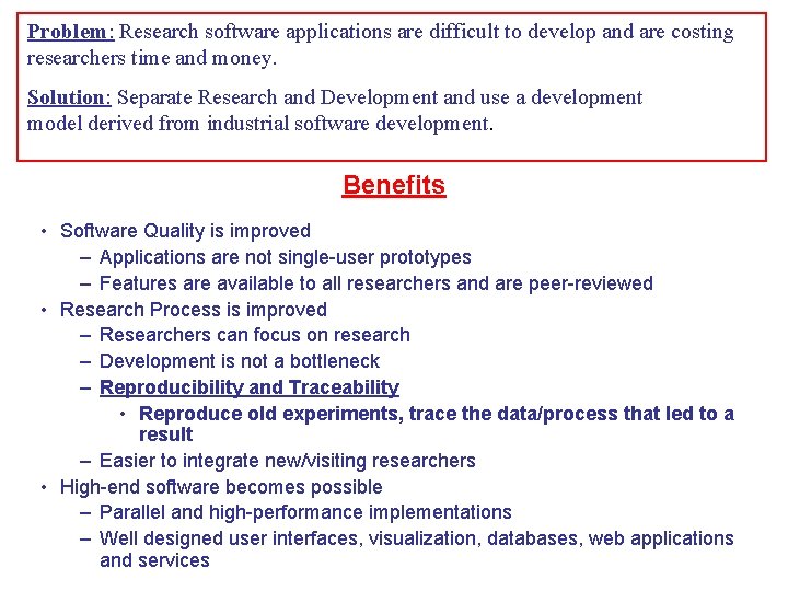
Problem: Research software applications are difficult to develop and are costing researchers time and money. Solution: Separate Research and Development and use a development model derived from industrial software development. Benefits • Software Quality is improved – Applications are not single-user prototypes – Features are available to all researchers and are peer-reviewed • Research Process is improved – Researchers can focus on research – Development is not a bottleneck – Reproducibility and Traceability • Reproduce old experiments, trace the data/process that led to a result – Easier to integrate new/visiting researchers • High-end software becomes possible – Parallel and high-performance implementations – Well designed user interfaces, visualization, databases, web applications and services

Compu. Cell 3 D collaboration University of Notre Dame , Indiana University People: Mark Alber, Ariel Balter, Rajiv Chaturvedi, Nan Chen, Trevor Cickovski, Jeff Coffland, Michael Crocker, Gabor Forgacs, James Glazier, Tilmann Glimm, George Hentschel, Chengbang Huang, Jesus Izaguirre, Chris Mueller, Stuart Newman, Nikodem Poplawski, Maciej Swat, Gilberto Thomas Funding agencies and institutions: NSF, ICSB Notre Dame, The Biocomplexity Institute Indiana University, NIH Users – most important part of the collaboration. Website: http: //sourceforge. net/projects/compucell/ Google keyword: Compu. Cell 3 D

Running the simulation Steering bar allows users to start or pause the simulation, zoom in , zoom out, to switch between 2 D and 3 D visualization, change view modes (cell field, pressure field , chemical concentration field, velocity field etc. . ) Player can output multiple views during single simulation run – Add Screenshot function Information bar

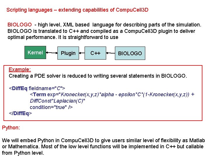
Scripting languages – extending capabilities of Compu. Cell 3 D BIOLOGO - high level, XML based language for describing parts of the simulation. BIOLOGO is translated to C++ and compiled as a Compu. Cell 3 D plugin to deliver optimal performance. It is straightforward to use Kernel Plugin C++ BIOLOGO Example: Creating a PDE solver is reduced to writing several statements in BIOLOGO. <Diff. Eq fieldname="C"> <Term exp="Kronecker(x, y, z)*alpha - epsilon*C*(1 -Kronecker(x, y, z)) + Diff. Const*Laplacian(C)" condition="true" /> </Diff. Eq> Python: We will embed Python in Compu. Cell 3 D to give users similar level of flexibility as Matlab or Mathematica. Most of the low level functions will be implemented in C++ but callable from Python level.

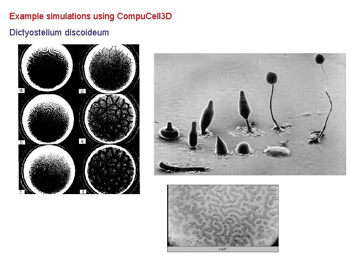
Example simulations using Compu. Cell 3 D Dictyostelium discoideum

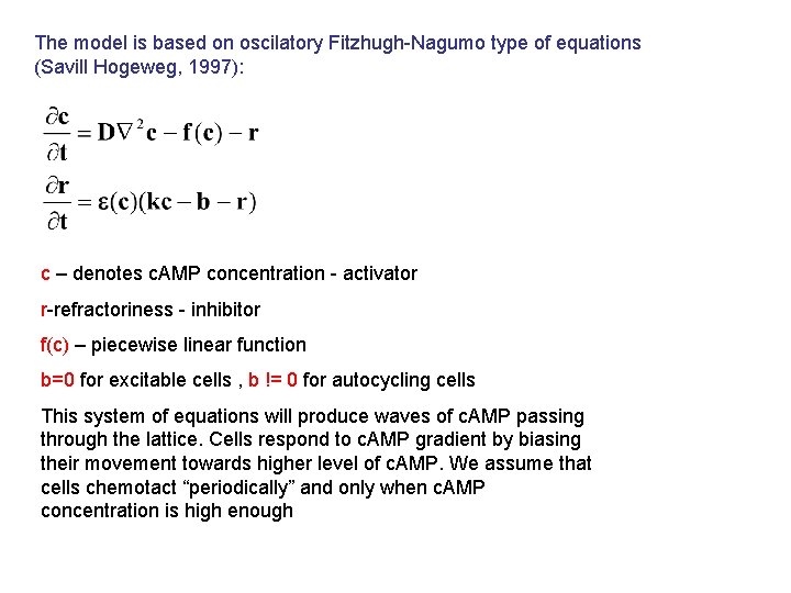
The model is based on oscilatory Fitzhugh-Nagumo type of equations (Savill Hogeweg, 1997): c – denotes c. AMP concentration - activator r-refractoriness - inhibitor f(c) – piecewise linear function b=0 for excitable cells , b != 0 for autocycling cells This system of equations will produce waves of c. AMP passing through the lattice. Cells respond to c. AMP gradient by biasing their movement towards higher level of c. AMP. We assume that cells chemotact “periodically” and only when c. AMP concentration is high enough

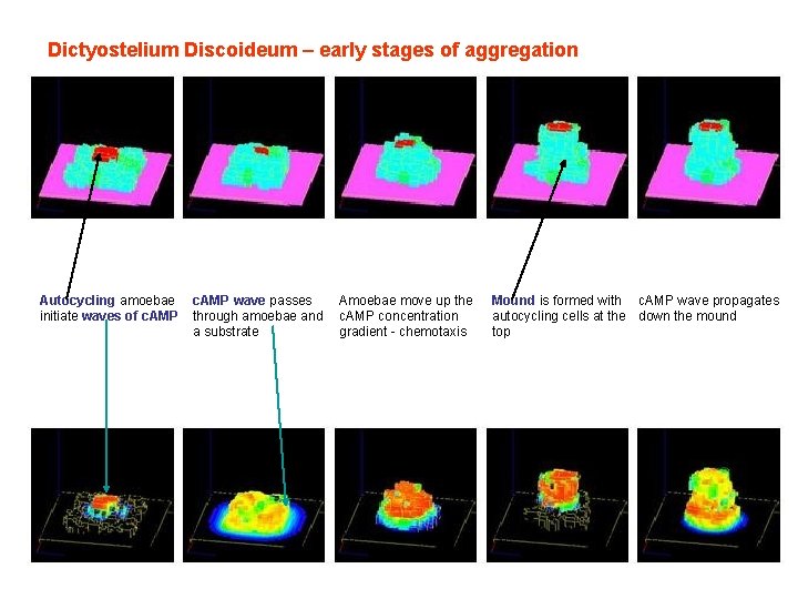
Dictyostelium Discoideum – early stages of aggregation Autocycling amoebae initiate waves of c. AMP wave passes through amoebae and a substrate Amoebae move up the c. AMP concentration gradient - chemotaxis Mound is formed with c. AMP wave propagates autocycling cells at the down the mound top

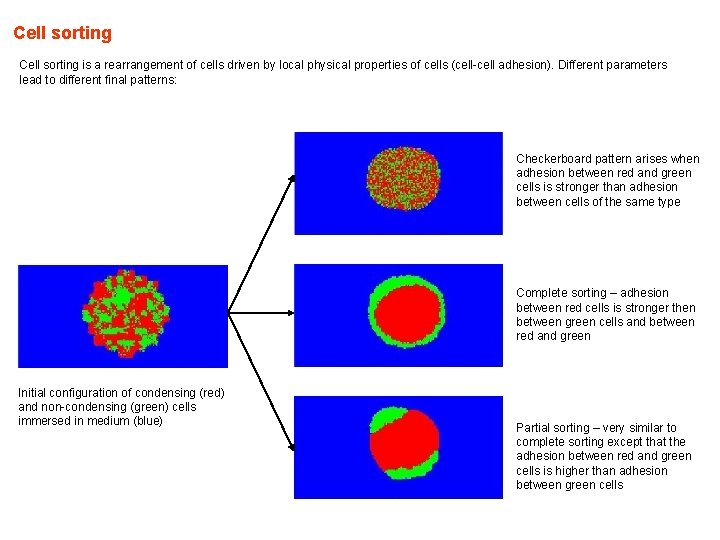
Cell sorting is a rearrangement of cells driven by local physical properties of cells (cell-cell adhesion). Different parameters lead to different final patterns: Checkerboard pattern arises when adhesion between red and green cells is stronger than adhesion between cells of the same type Complete sorting – adhesion between red cells is stronger then between green cells and between red and green Initial configuration of condensing (red) and non-condensing (green) cells immersed in medium (blue) Partial sorting – very similar to complete sorting except that the adhesion between red and green cells is higher than adhesion between green cells

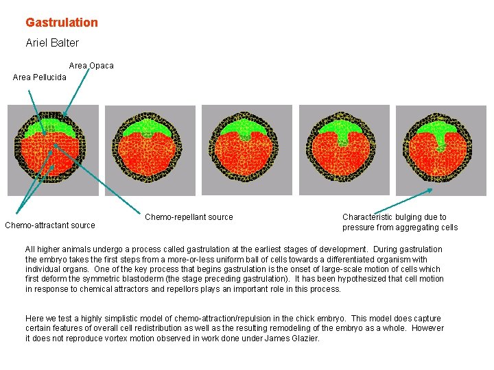
Gastrulation Ariel Balter Area Opaca Area Pellucida Chemo-attractant source Chemo-repellant source Characteristic bulging due to pressure from aggregating cells All higher animals undergo a process called gastrulation at the earliest stages of development. During gastrulation the embryo takes the first steps from a more-or-less uniform ball of cells towards a differentiated organism with individual organs. One of the key process that begins gastrulation is the onset of large-scale motion of cells which first deform the symmetric blastoderm (the stage preceding gastrulation). It has been hypothesized that cell motion in response to chemical attractors and repellors plays an important role in this process. Here we test a highly simplistic model of chemo-attraction/repulsion in the chick embryo. This model does capture certain features of overall cell redistribution as well as the resulting remodeling of the embryo as a whole. However it does not reproduce vortex motion observed in work done under James Glazier.

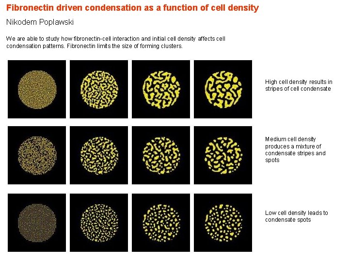
Fibronectin driven condensation as a function of cell density Nikodem Poplawski We are able to study how fibronectin-cell interaction and initial cell density affects cell condensation patterns. Fibronectin limits the size of forming clusters. High cell density results in stripes of cell condensate Medium cell density produces a mixture of condensate stripes and spots Low cell density leads to condensate spots

Roadmap Compu. Cell 3 D needs further development in order to become a universal framework for modeling morphogenesis: 1 st quarter 2006 -Full support for scripting languages -Isolate users from XML - graphical configuration tools -Provide full diagnostics of the simulation in Compu. Cell Player – for example rightclick should provide information about given cell 2 nd-3 rd quarter 2006 -Movies, scientific plots and all lattice information will be available through the Player -Parallel version 2006/2007 -Steering and parameters sweeps -Serializing simulation – users will be able to stop the simulaiton and resume it later -Project management