Introduction to Compu Cell 3 D Maciej Swat

Introduction to Compu. Cell 3 D Maciej Swat Biocomplexity Institute Indiana University Bloomington, IN 47405 USA Developing Multi-Scale, Multicell Developmental and Biomedical Simulations with Compu. Cell 3 D RTP, NC, 2012 July 30 th-August 3 rd 2012 IU Team: Susan Hester, Julio Belmonte, Abbas Shirinifard, Ryan Roper, Alin Comanescu, Benjamin Zaitlen, Randy Heiland, Dr. Dragos Amarie, Dr. Scott Gens, Dr. James A. Glazier, Dr. James Sluka, Dr. Sherry Clendenon, Dr. Mitja Hmeljak, Dr. Srividhya Jayaraman, Dr. Gilberto Thomas Support: EPA, NIH/NIGMS, NAKFI, Indiana University

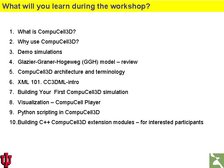
What will you learn during the workshop? 1. What is Compu. Cell 3 D? 2. Why use Compu. Cell 3 D? 3. Demo simulations 4. Glazier-Graner-Hogeweg (GGH) model – review 5. Compu. Cell 3 D architecture and terminology 6. XML 101. CC 3 DML-intro 7. Building Your First Compu. Cell 3 D simulation 8. Visualization – Compu. Cell Player 9. Python scripting in Compu. Cell 3 D 10. Building C++ Compu. Cell 3 D extension modules – for interested participants

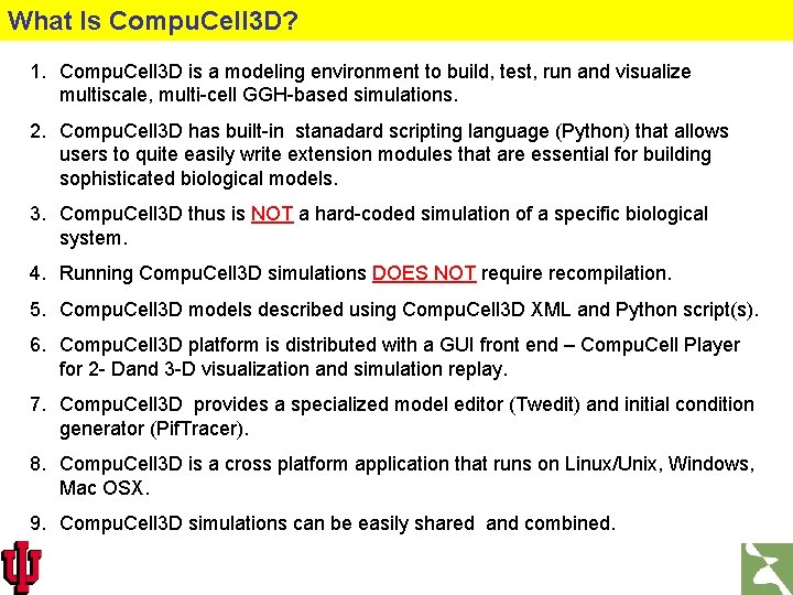
What Is Compu. Cell 3 D? 1. Compu. Cell 3 D is a modeling environment to build, test, run and visualize multiscale, multi-cell GGH-based simulations. 2. Compu. Cell 3 D has built-in stanadard scripting language (Python) that allows users to quite easily write extension modules that are essential for building sophisticated biological models. 3. Compu. Cell 3 D thus is NOT a hard-coded simulation of a specific biological system. 4. Running Compu. Cell 3 D simulations DOES NOT require recompilation. 5. Compu. Cell 3 D models described using Compu. Cell 3 D XML and Python script(s). 6. Compu. Cell 3 D platform is distributed with a GUI front end – Compu. Cell Player for 2 - Dand 3 -D visualization and simulation replay. 7. Compu. Cell 3 D provides a specialized model editor (Twedit) and initial condition generator (Pif. Tracer). 8. Compu. Cell 3 D is a cross platform application that runs on Linux/Unix, Windows, Mac OSX. 9. Compu. Cell 3 D simulations can be easily shared and combined.

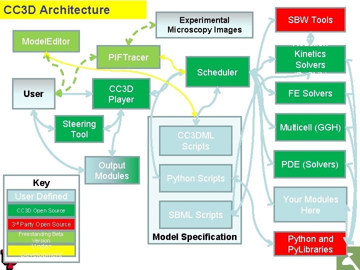
CC 3 D Architecture Experimental Microscopy Images Model. Editor PIFTracer Scheduler CC 3 D Player User Steering Tool Key User Defined CC 3 D Open Source 3 rd Output Modules SBW Tools Reaction Kinetics Solvers (So. SLib) FE Solvers CC 3 DML Scripts Multicell (GGH) PDE (Solvers) Python Scripts SBML Scripts Your Modules Here Party Open Source Freestanding Beta Version Under Development Model Specification Python and Py. Libraries

Why Use Compu. Cell 3 D? What Are the Alternatives? 1. Compu. Cell 3 D allows users to set up and run their simulations in minutes to hours rather than weeks to months for custom code. 2. Most Compu. Cell 3 D simulations DO NOT need to be recompiled. To change parameters (in XML or Python scripts) or logic (in Python scripts) you just make the changes in the script or on the fly and run. Recompilation of hard-coded simulation is error prone and is accessible only to users with significant programming background. 3. Compu. Cell 3 D is actively developed , maintained and supported. The www. compucell 3 d. org website provides manuals, tutorials and developer documentation. Compu. Cell 3 D has approx. 4 releases each year. 4. Compu. Cell 3 D has many users around the world, faciltiating collaboration and module exchange, saving time when developing new models. 5. The Biocomplexity Institute organizes training workshops and mentorship programs. Those are great opportunities to learn biological modeling using Compu. Cell 3 D. For more info see www. compucell 3 d. org

Why are model sharing and standards important? 1. 99% of modeling done with custom written code is hard or impossible to reproduce or verify. In publications , even ones including full code listings, authors often forget to describe details which are essential to reproducing their described work. 2. Using standard modeling tools improves the chances of your research being accepted and further refined by other scientists. 3. Standards allow people to spend more time working on new ideas and less struggling to reproduce old results. 4. Standards greatly improves research efficiency. 5. Bug tracking and detection are much more efficient with shared tools than with custom written ones. Bugs are also better documented for shared software. 6. Developing and sharing modules with other researchers is the best way to improve software modeling tools used by the research community.

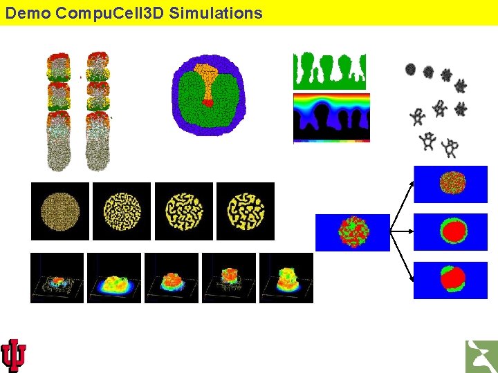
Demo Compu. Cell 3 D Simulations

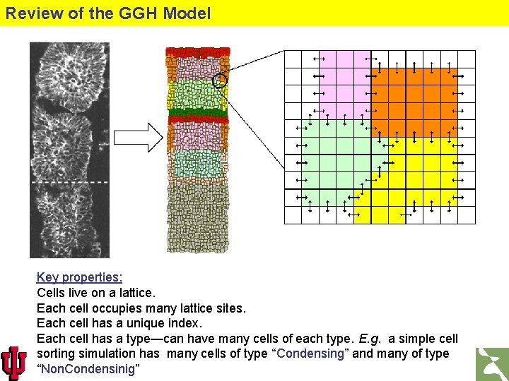
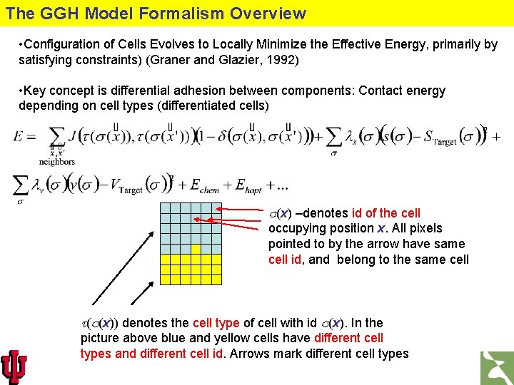
Review of the GGH Model Key properties: Cells live on a lattice. Each cell occupies many lattice sites. Each cell has a unique index. Each cell has a type—can have many cells of each type. E. g. a simple cell sorting simulation has many cells of type “Condensing” and many of type “Non. Condensinig”

The GGH Model Formalism Overview • Configuration of Cells Evolves to Locally Minimize the Effective Energy, primarily by satisfying constraints) (Graner and Glazier, 1992) • Key concept is differential adhesion between components: Contact energy depending on cell types (differentiated cells) s(x) –denotes id of the cell occupying position x. All pixels pointed to by the arrow have same cell id, and belong to the same cell t(s(x)) denotes the cell type of cell with id s(x). In the picture above blue and yellow cells have different cell types and different cell id. Arrows mark different cell types

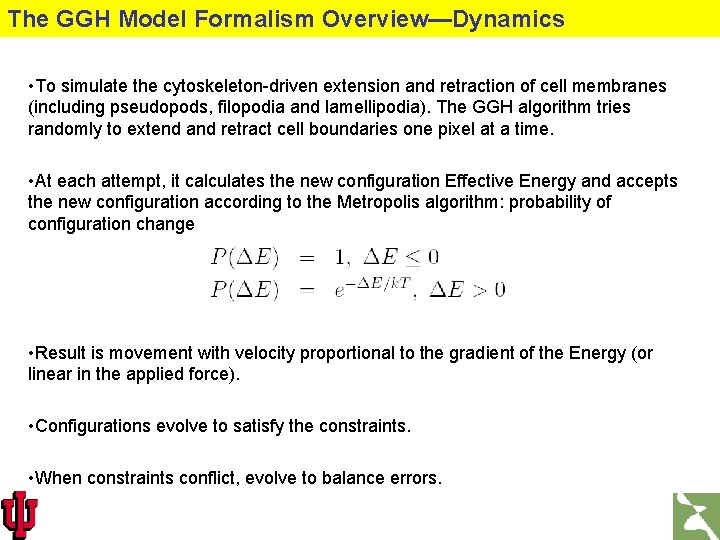
The GGH Model Formalism Overview—Dynamics • To simulate the cytoskeleton-driven extension and retraction of cell membranes (including pseudopods, filopodia and lamellipodia). The GGH algorithm tries randomly to extend and retract cell boundaries one pixel at a time. • At each attempt, it calculates the new configuration Effective Energy and accepts the new configuration according to the Metropolis algorithm: probability of configuration change • Result is movement with velocity proportional to the gradient of the Energy (or linear in the applied force). • Configurations evolve to satisfy the constraints. • When constraints conflict, evolve to balance errors.

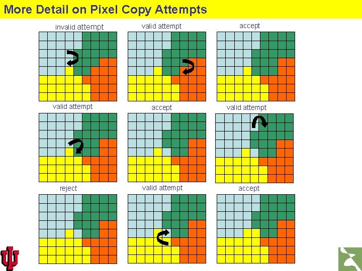
More Detail on Pixel Copy Attempts invalid attempt reject valid attempt accept

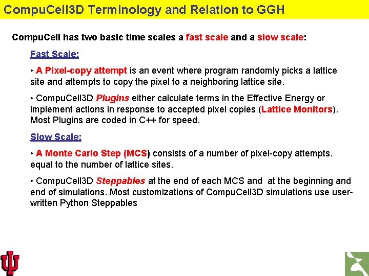
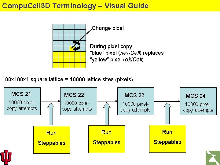
Compu. Cell 3 D Terminology and Relation to GGH Compu. Cell has two basic time scales a fast scale and a slow scale: Fast Scale: • A Pixel-copy attempt is an event where program randomly picks a lattice site and attempts to copy the pixel to a neighboring lattice site. • Compu. Cell 3 D Plugins either calculate terms in the Effective Energy or implement actions in response to accepted pixel copies (Lattice Monitors). Most Plugins are coded in C++ for speed. Slow Scale: • A Monte Carlo Step (MCS) consists of a number of pixel-copy attempts. equal to the number of lattice sites. • Compu. Cell 3 D Steppables at the end of each MCS and at the beginning and end of simulations. Most customizations of Compu. Cell 3 D simulations userwritten Python Steppables

Compu. Cell 3 D Terminology – Visual Guide Change pixel During pixel copy “blue” pixel (new. Cell) replaces “yellow” pixel (old. Cell) 100 x 1 square lattice = 10000 lattice sites (pixels) MCS 21 MCS 22 10000 pixelcopy attempts MCS 23 10000 pixelcopy attempts MCS 24 10000 pixelcopy attempts Run Run Steppables

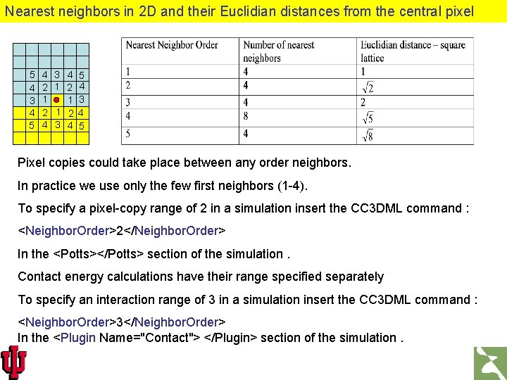
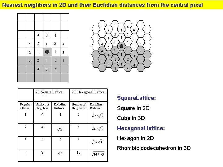
Nearest neighbors in 2 D and their Euclidian distances from the central pixel 5 4 3 4 5 4 2 1 2 4 3 4 5 1 2 4 1 3 1 2 4 3 4 5 Pixel copies could take place between any order neighbors. In practice we use only the few first neighbors (1 -4). To specify a pixel-copy range of 2 in a simulation insert the CC 3 DML command : <Neighbor. Order>2</Neighbor. Order> In the <Potts></Potts> section of the simulation. Contact energy calculations have their range specified separately To specify an interaction range of 3 in a simulation insert the CC 3 DML command : <Neighbor. Order>3</Neighbor. Order> In the <Plugin Name="Contact"> </Plugin> section of the simulation.

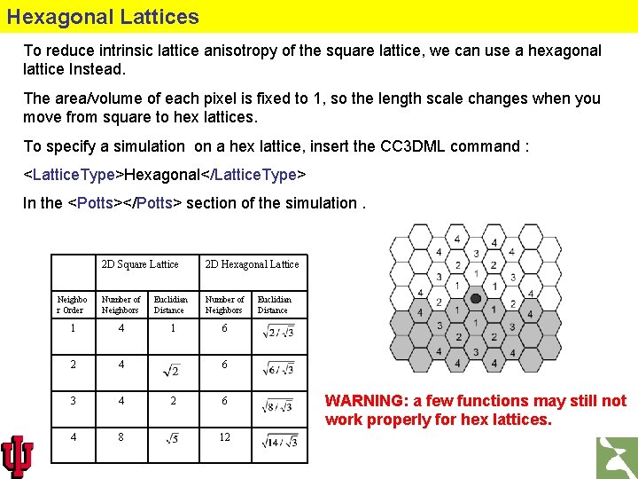
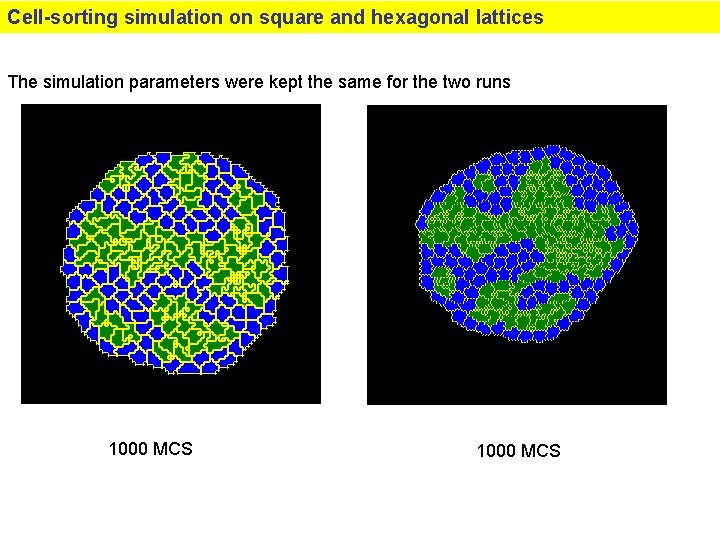
Hexagonal Lattices To reduce intrinsic lattice anisotropy of the square lattice, we can use a hexagonal lattice Instead. The area/volume of each pixel is fixed to 1, so the length scale changes when you move from square to hex lattices. To specify a simulation on a hex lattice, insert the CC 3 DML command : <Lattice. Type>Hexagonal</Lattice. Type> In the <Potts></Potts> section of the simulation. 2 D Square Lattice 2 D Hexagonal Lattice Neighbo r Order Number of Neighbors Euclidian Distance Number of Neighbors 1 4 1 6 2 4 3 4 4 8 Euclidian Distance 6 2 6 12 WARNING: a few functions may still not work properly for hex lattices.

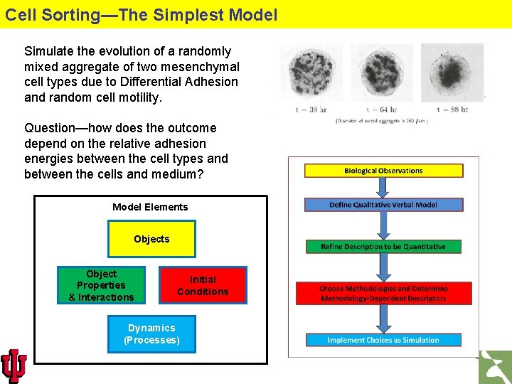
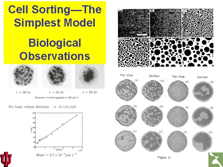
Cell Sorting—The Simplest Model Simulate the evolution of a randomly mixed aggregate of two mesenchymal cell types due to Differential Adhesion and random cell motility. Question—how does the outcome depend on the relative adhesion energies between the cell types and between the cells and medium? Model Elements Object Properties & Interactions Initial Conditions Dynamics (Processes) 16

Cell Sorting—The Simplest Model Biological Observations

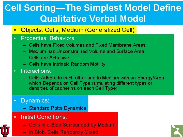
Cell Sorting—The Simplest Model Define Qualitative Verbal Model • Objects: Cells, Medium (Generalized Cell) • Properties, Behaviors: – – Cells have Fixed Volumes and Fixed Membrane Areas Medium has Unconstrained Volume and Surface Area Cells are Adhesive Cells have Intrinsic Random Motility • Interactions: – Cells Adhere to each other and to Medium with an Energy/Area which Depends on Cell Type (simulating different types or densities of cadherins on each Cell Type) • Dynamics: – Standard Potts Dynamics • Initial Conditions: – Cells in a Blob Surrounded by Medium – In Blob, Cells Randomly Mixed

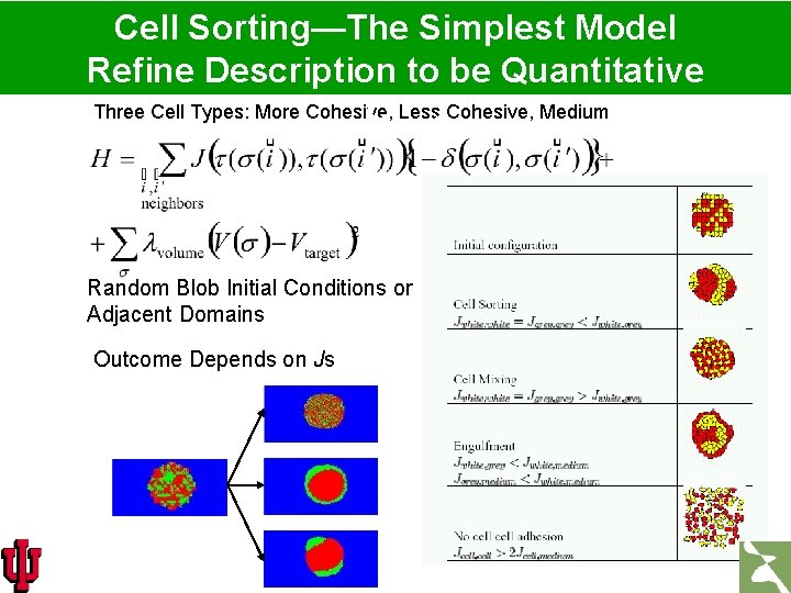
Cell Sorting—The Simplest Model Refine Description to be Quantitative Three Cell Types: More Cohesive, Less Cohesive, Medium Random Blob Initial Conditions or Adjacent Domains Outcome Depends on Js

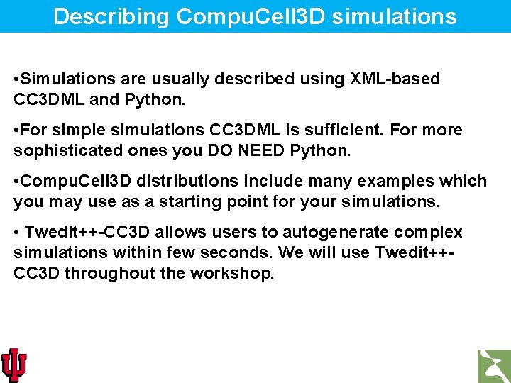
Describing Compu. Cell 3 D simulations • Simulations are usually described using XML-based CC 3 DML and Python. • For simple simulations CC 3 DML is sufficient. For more sophisticated ones you DO NEED Python. • Compu. Cell 3 D distributions include many examples which you may use as a starting point for your simulations. • Twedit++-CC 3 D allows users to autogenerate complex simulations within few seconds. We will use Twedit++CC 3 D throughout the workshop.

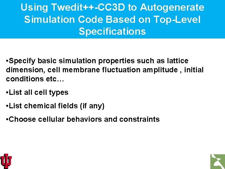
Using Twedit++-CC 3 D to Autogenerate Simulation Code Based on Top-Level Specifications • Specify basic simulation properties such as lattice dimension, cell membrane fluctuation amplitude , initial conditions etc… • List all cell types • List chemical fields (if any) • Choose cellular behaviors and constraints

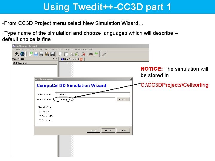
Using Twedit++-CC 3 D part 1 • From CC 3 D Project menu select New Simulation Wizard… • Type name of the simulation and choose languages which will describe – default choice is fine NOTICE: The simulation will be stored in C: CC 3 DProjectsCellsorting

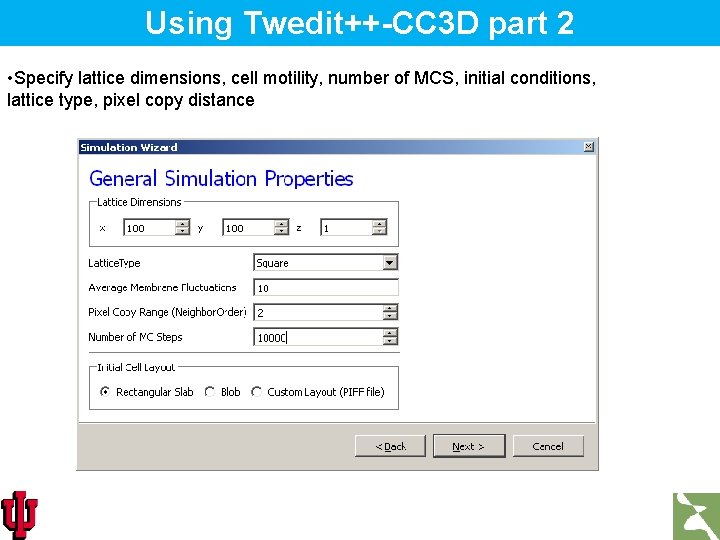
Using Twedit++-CC 3 D part 2 • Specify lattice dimensions, cell motility, number of MCS, initial conditions, lattice type, pixel copy distance

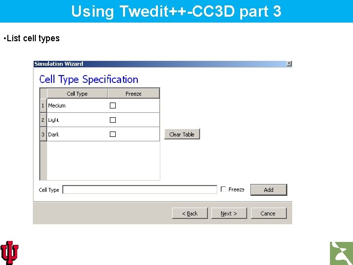
Using Twedit++-CC 3 D part 3 • List cell types

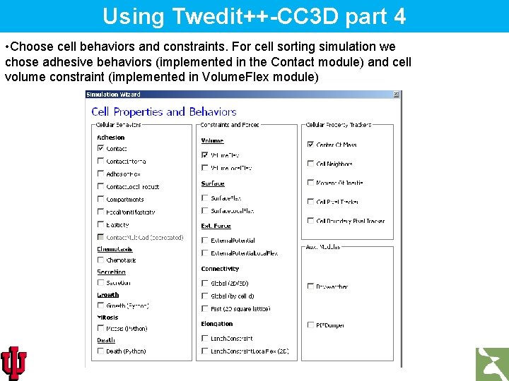
Using Twedit++-CC 3 D part 4 • Choose cell behaviors and constraints. For cell sorting simulation we chose adhesive behaviors (implemented in the Contact module) and cell volume constraint (implemented in Volume. Flex module)

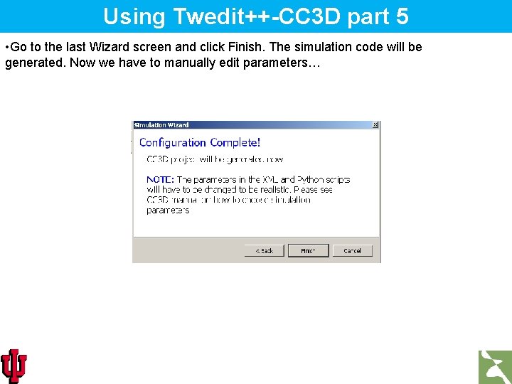
Using Twedit++-CC 3 D part 5 • Go to the last Wizard screen and click Finish. The simulation code will be generated. Now we have to manually edit parameters…

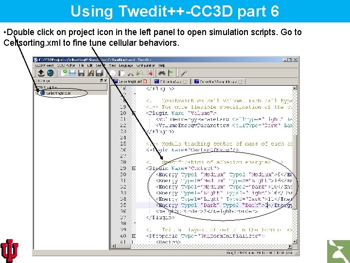
Using Twedit++-CC 3 D part 6 • Double click on project icon in the left panel to open simulation scripts. Go to Cellsorting. xml to fine tune cellular behaviors.

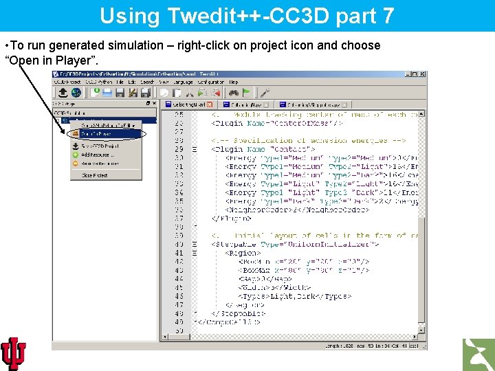
Using Twedit++-CC 3 D part 7 • To run generated simulation – right-click on project icon and choose “Open in Player”.

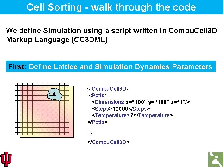
Cell Sorting - walk through the code We define Simulation using a script written in Compu. Cell 3 D Markup Language (CC 3 DML) First: Define Lattice and Simulation Dynamics Parameters Cell < Compu. Cell 3 D> <Potts> <Dimensions x=“ 100" y=“ 100" z=“ 1"/> <Steps>10000</Steps> <Temperature>2</Temperature> </Potts> … </Compu. Cell 3 D>

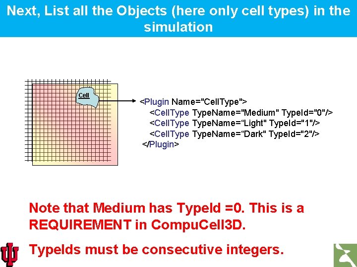
Next, List all the Objects (here only cell types) in the simulation Cell <Plugin Name="Cell. Type"> <Cell. Type. Name="Medium" Type. Id="0"/> <Cell. Type. Name=“Light" Type. Id="1"/> <Cell. Type. Name=“Dark" Type. Id="2"/> </Plugin> Note that Medium has Type. Id =0. This is a REQUIREMENT in Compu. Cell 3 D. Type. Ids must be consecutive integers.

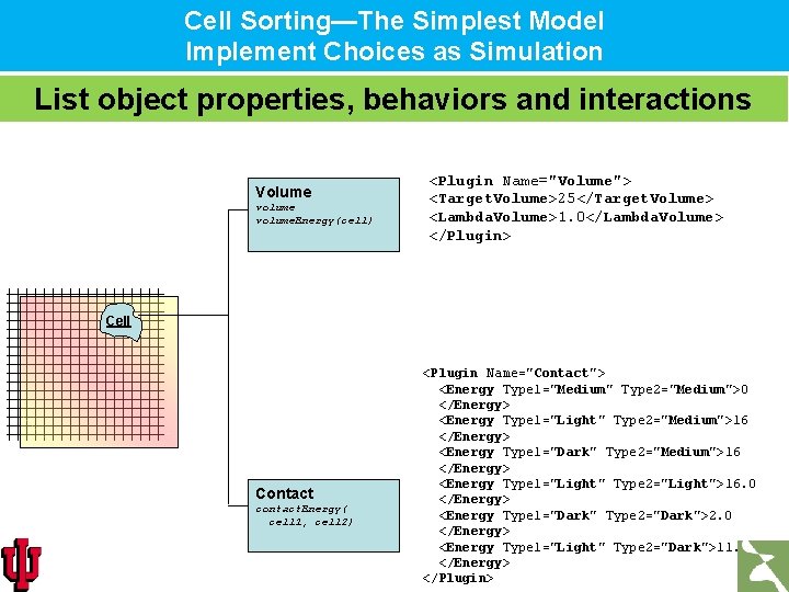
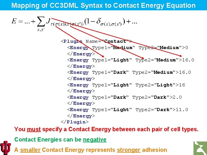
Cell Sorting—The Simplest Model Implement Choices as Simulation List object properties, behaviors and interactions Volume volume. Energy(cell) <Plugin Name="Volume"> <Target. Volume>25</Target. Volume> <Lambda. Volume>1. 0</Lambda. Volume> </Plugin> Cell Contact contact. Energy( cell 1, cell 2) <Plugin Name="Contact"> <Energy Type 1="Medium" Type 2="Medium">0 </Energy> <Energy Type 1="Light" Type 2="Medium">16 </Energy> <Energy Type 1="Dark" Type 2="Medium">16 </Energy> <Energy Type 1="Light" Type 2="Light">16. 0 </Energy> <Energy Type 1="Dark" Type 2="Dark">2. 0 </Energy> <Energy Type 1="Light" Type 2="Dark">11. 0 </Energy> </Plugin>

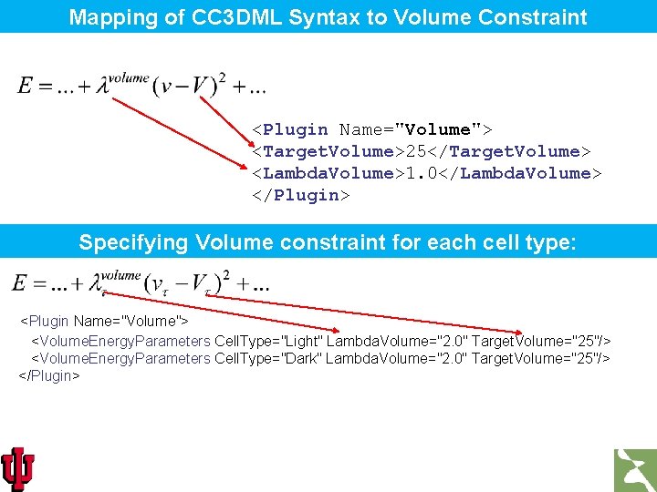
Mapping of CC 3 DML Syntax to Volume Constraint <Plugin Name="Volume"> <Target. Volume>25</Target. Volume> <Lambda. Volume>1. 0</Lambda. Volume> </Plugin> Specifying Volume constraint for each cell type: <Plugin Name="Volume"> <Volume. Energy. Parameters Cell. Type="Light" Lambda. Volume="2. 0" Target. Volume="25"/> <Volume. Energy. Parameters Cell. Type="Dark" Lambda. Volume="2. 0" Target. Volume="25"/> </Plugin>

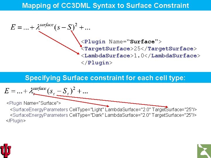
Mapping of CC 3 DML Syntax to Surface Constraint <Plugin Name=“Surface"> <Target. Surface>25</Target. Surface> <Lambda. Surface>1. 0</Lambda. Surface> </Plugin> Specifying Surface constraint for each cell type: <Plugin Name=“Surface"> <Surface. Energy. Parameters Cell. Type="Light" Lambda. Surface="2. 0" Target. Surface="25"/> <Surface. Energy. Parameters Cell. Type="Dark" Lambda. Surface="2. 0" Target. Surface="25"/> </Plugin>

Mapping of CC 3 DML Syntax to Contact Energy Equation <Plugin Name="Contact"> <Energy Type 1="Medium" Type 2="Medium">0 </Energy> <Energy Type 1="Light" Type 2="Medium">16. 0 </Energy> <Energy Type 1="Dark" Type 2="Medium">16. 0 </Energy> <Energy Type 1="Light" Type 2="Light">16 </Energy> <Energy Type 1="Dark" Type 2="Dark">2. 0 </Energy> <Energy Type 1="Light" Type 2="Dark">11. 0 </Energy> </Plugin> You must specify a Contact Energy between each pair of cell types. Contact Energies can be negative A smaller Contact Energy represents stronger adhesion

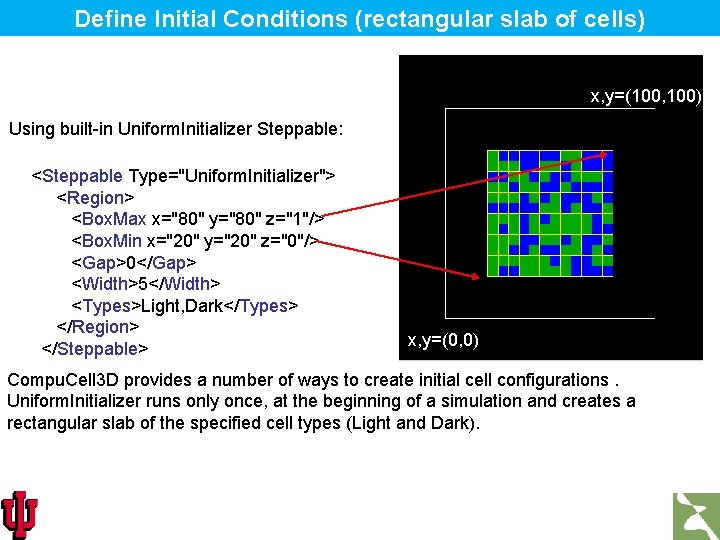
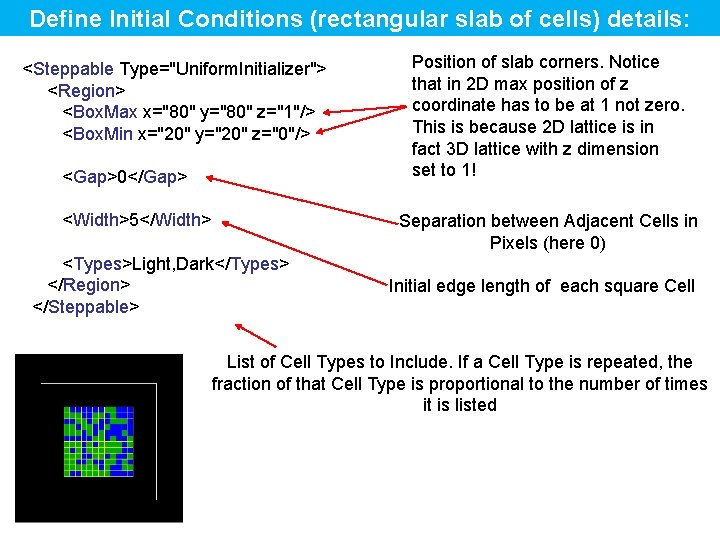
Define Initial Conditions (rectangular slab of cells) x, y=(100, 100) Using built-in Uniform. Initializer Steppable: <Steppable Type="Uniform. Initializer"> <Region> <Box. Max x="80" y="80" z="1"/> <Box. Min x="20" y="20" z="0"/> <Gap>0</Gap> <Width>5</Width> <Types>Light, Dark</Types> </Region> </Steppable> x, y=(0, 0) Compu. Cell 3 D provides a number of ways to create initial cell configurations. Uniform. Initializer runs only once, at the beginning of a simulation and creates a rectangular slab of the specified cell types (Light and Dark).

Define Initial Conditions (rectangular slab of cells) details: <Steppable Type="Uniform. Initializer"> <Region> <Box. Max x="80" y="80" z="1"/> <Box. Min x="20" y="20" z="0"/> <Gap>0</Gap> <Width>5</Width> Position of slab corners. Notice that in 2 D max position of z coordinate has to be at 1 not zero. This is because 2 D lattice is in fact 3 D lattice with z dimension set to 1! Separation between Adjacent Cells in Pixels (here 0) <Types>Light, Dark</Types> </Region> </Steppable> Initial edge length of each square Cell List of Cell Types to Include. If a Cell Type is repeated, the fraction of that Cell Type is proportional to the number of times it is listed

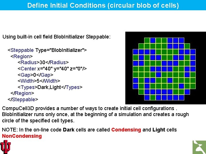
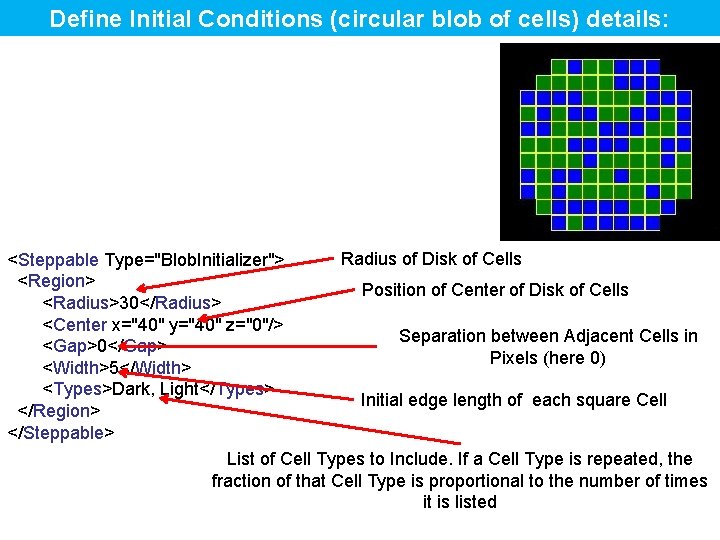
Define Initial Conditions (circular blob of cells) Using built-in cell field Blob. Initializer Steppable: <Steppable Type="Blob. Initializer"> <Region> <Radius>30</Radius> <Center x="40" y="40" z="0"/> <Gap>0</Gap> <Width>5</Width> <Types>Dark, Light</Types> </Region> </Steppable> Compu. Cell 3 D provides a number of ways to create initial cell configurations. Blob. Initializer runs only once, at the beginning of a simulation and creates a rough circle of the specified cell types. NOTE: In the on-line code Dark cells are called Condensing and Light cells Non. Condensing

Define Initial Conditions (circular blob of cells) details: Radius of Disk of Cells <Steppable Type="Blob. Initializer"> <Region> Position of Center of Disk of Cells <Radius>30</Radius> <Center x="40" y="40" z="0"/> Separation between Adjacent Cells in <Gap>0</Gap> Pixels (here 0) <Width>5</Width> <Types>Dark, Light</Types> Initial edge length of each square Cell </Region> </Steppable> List of Cell Types to Include. If a Cell Type is repeated, the fraction of that Cell Type is proportional to the number of times it is listed

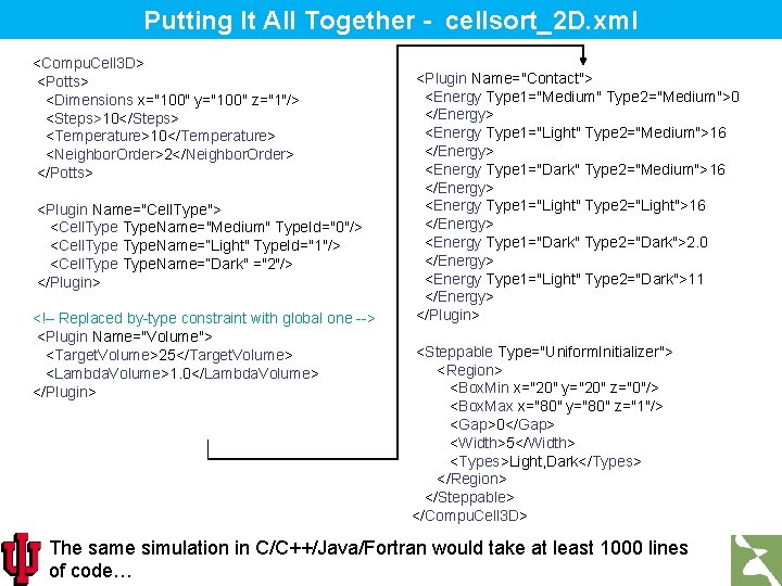
Putting It All Together - cellsort_2 D. xml <Compu. Cell 3 D> <Potts> <Dimensions x="100" y="100" z="1"/> <Steps>10</Steps> <Temperature>10</Temperature> <Neighbor. Order>2</Neighbor. Order> </Potts> <Plugin Name="Cell. Type"> <Cell. Type. Name="Medium" Type. Id="0"/> <Cell. Type. Name=“Light" Type. Id="1"/> <Cell. Type. Name=“Dark" ="2"/> </Plugin> <!– Replaced by-type constraint with global one --> <Plugin Name="Volume"> <Target. Volume>25</Target. Volume> <Lambda. Volume>1. 0</Lambda. Volume> </Plugin> <Plugin Name="Contact"> <Energy Type 1="Medium" Type 2="Medium">0 </Energy> <Energy Type 1="Light" Type 2="Medium">16 </Energy> <Energy Type 1="Dark" Type 2="Medium">16 </Energy> <Energy Type 1="Light" Type 2="Light">16 </Energy> <Energy Type 1="Dark" Type 2="Dark">2. 0 </Energy> <Energy Type 1="Light" Type 2="Dark">11 </Energy> </Plugin> <Steppable Type="Uniform. Initializer"> <Region> <Box. Min x="20" y="20" z="0"/> <Box. Max x="80" y="80" z="1"/> <Gap>0</Gap> <Width>5</Width> <Types>Light, Dark</Types> </Region> </Steppable> </Compu. Cell 3 D> The same simulation in C/C++/Java/Fortran would take at least 1000 lines of code…

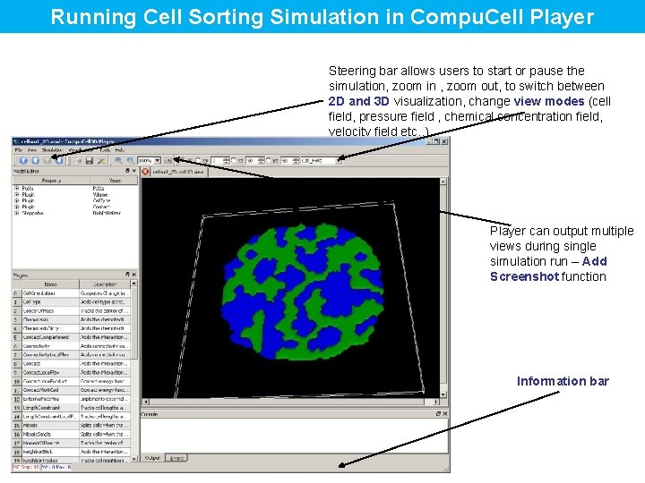
Running Cell Sorting Simulation in Compu. Cell Player Steering bar allows users to start or pause the simulation, zoom in , zoom out, to switch between 2 D and 3 D visualization, change view modes (cell field, pressure field , chemical concentration field, velocity field etc. . ) Player can output multiple views during single simulation run – Add Screenshot function Information bar

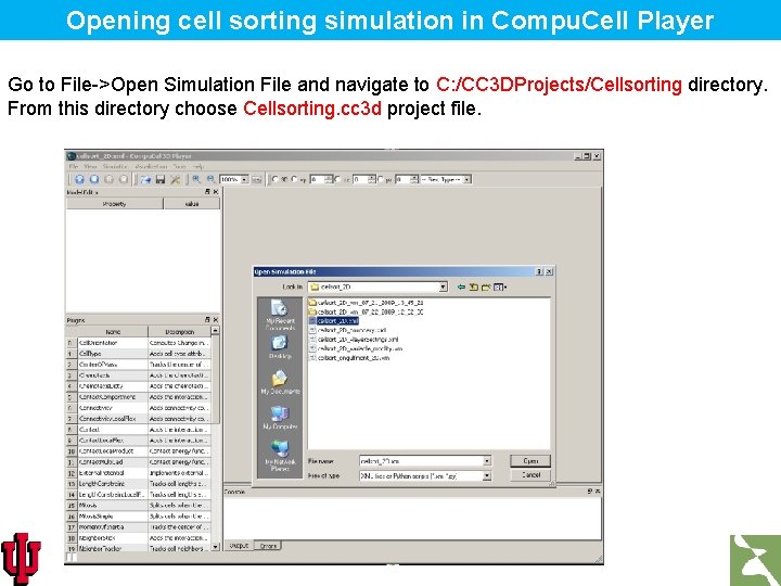
Opening cell sorting simulation in Compu. Cell Player Go to File->Open Simulation File and navigate to C: /CC 3 DProjects/Cellsorting directory. From this directory choose Cellsorting. cc 3 d project file.

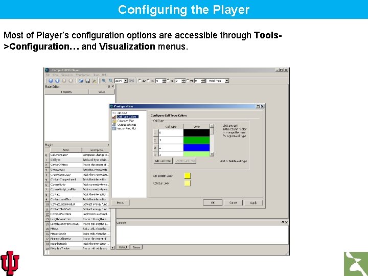
Configuring the Player Most of Player’s configuration options are accessible through Tools>Configuration… and Visualization menus.

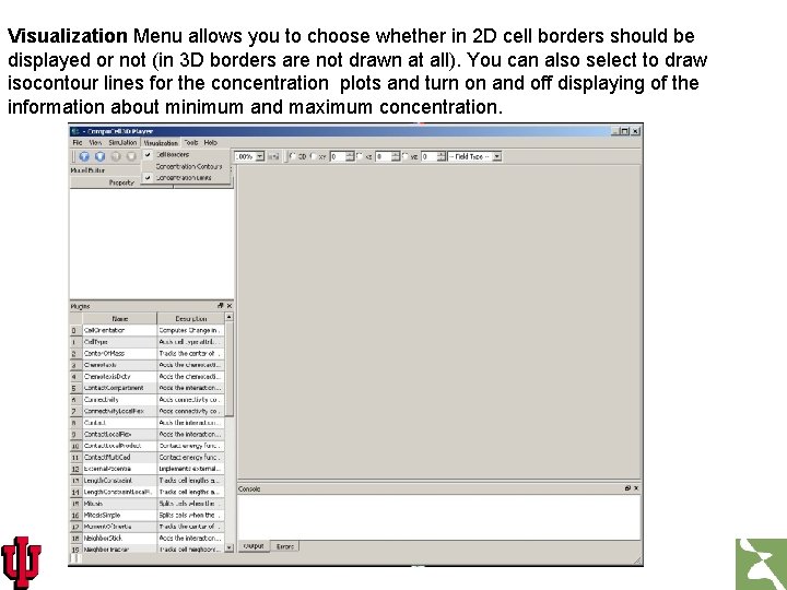
Visualization Menu allows you to choose whether in 2 D cell borders should be displayed or not (in 3 D borders are not drawn at all). You can also select to draw isocontour lines for the concentration plots and turn on and off displaying of the information about minimum and maximum concentration.

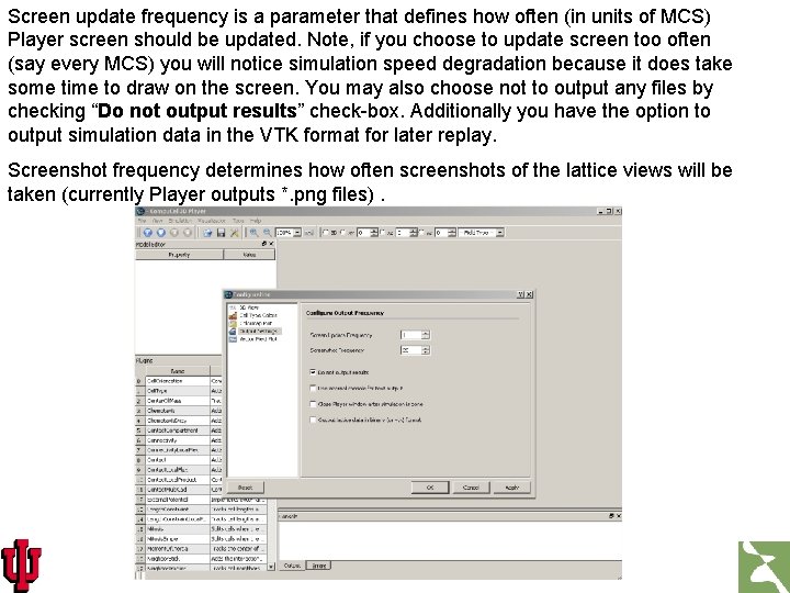
Screen update frequency is a parameter that defines how often (in units of MCS) Player screen should be updated. Note, if you choose to update screen too often (say every MCS) you will notice simulation speed degradation because it does take some time to draw on the screen. You may also choose not to output any files by checking “Do not output results” check-box. Additionally you have the option to output simulation data in the VTK format for later replay. Screenshot frequency determines how often screenshots of the lattice views will be taken (currently Player outputs *. png files).

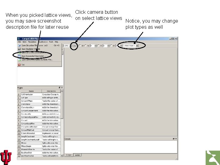
Screenshots are taken every “Screenshot Frequency” MCS By default Player will store screenshots of the currently displayed lattice view. In addition to this users can choose to store additional screenshots at the same time. Simply switch to different lattice view, click camera button. Those additional screenshots will be taken irrespectively of what Player currently displays. Once you selected additional screenshots it is convenient to save screenshot description file (it is written automatically by the Player, user just provide file name). Next time you decide to run Compu. Cell 3 D you may just use command compucell 3 d. sh -s screenshot. Desctiption. File_cellsort. txt -i cellsort_2 D. xml This will run simulation where stored screenshots will be taken

Click camera button When you picked lattice views, on select lattice views you may save screenshot Notice, you may change description file for later reuse plot types as well

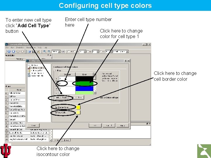
Configuring cell type colors To enter new cell type click “Add Cell Type” button Enter cell type number here Click here to change color for cell type 1 Click here to change cell border color Click here to change isocontour color

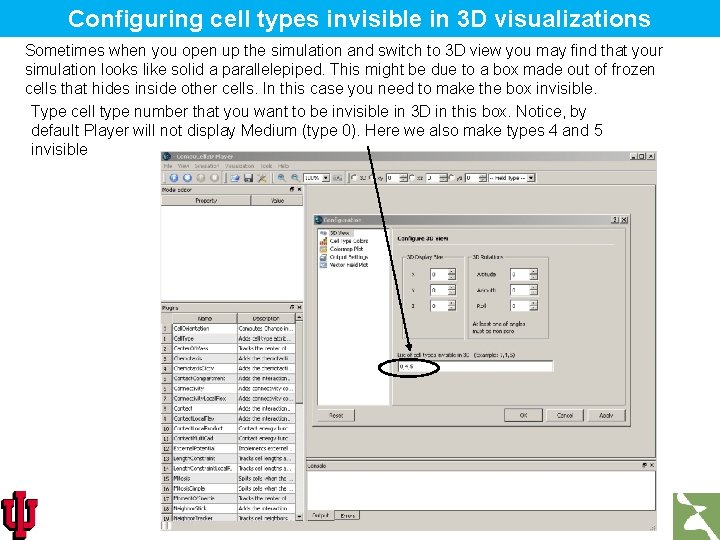
Configuring cell types invisible in 3 D visualizations Sometimes when you open up the simulation and switch to 3 D view you may find that your simulation looks like solid a parallelepiped. This might be due to a box made out of frozen cells that hides inside other cells. In this case you need to make the box invisible. Type cell type number that you want to be invisible in 3 D in this box. Notice, by default Player will not display Medium (type 0). Here we also make types 4 and 5 invisible

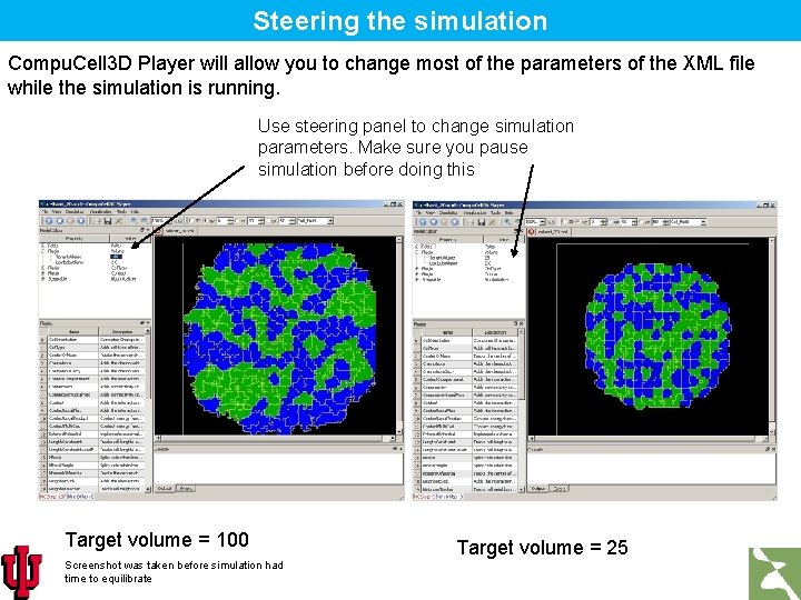
Steering the simulation Compu. Cell 3 D Player will allow you to change most of the parameters of the XML file while the simulation is running. Use steering panel to change simulation parameters. Make sure you pause simulation before doing this Target volume = 100 Screenshot was taken before simulation had time to equilibrate Target volume = 25

Exploring how different parameters affect cellular behaviors in cell sorting simulation 1. Vary cell membrane fluctuation amplitude (aka temperature) 2. Vary Lambda. Volume, Target. Volume 3. Vary Contact Energy coefficients Please refer to the Quick start guide to find set of exercises which will help you better understand the roles played by all parameters

Practical way of guessing contact energy hierarchy Basic facts: • Cells that have high contact energies between themselves, when they come together they increase overall energy of the system. Such cells tend to stay away from each other. • Cells that have low contact energies between themselves, when they come together they decrease overall energy of the system. Such cells tend to cluster together. • Those two rules are helpful when determining contact energy hierarchy. Simply cells of one type like to be surrounded by those cells with which the contact energy is the lowest. • And vice versa, if you want to make two cells not to touch each other, make sure that contact energy between them is high.

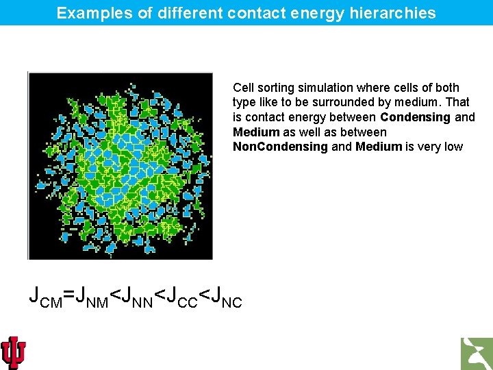
Examples of different contact energy hierarchies Cell sorting simulation where cells of both type like to be surrounded by medium. That is contact energy between Condensing and Medium as well as between Non. Condensing and Medium is very low JCM=JNM<JNN<JCC<JNC

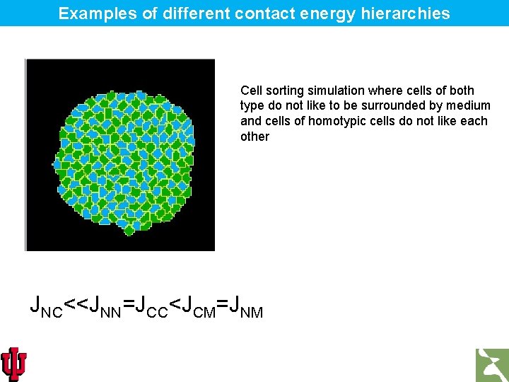
Examples of different contact energy hierarchies Cell sorting simulation where cells of both type do not like to be surrounded by medium and cells of homotypic cells do not like each other JNC<<JNN=JCC<JCM=JNM

Compu. Cell 3 D Subtleties Now that we’ve seen and run a simulation, we can go back and review some general points: 1. Understanding XML 2. Running CC 3 D from command line (useful for running CC 3 D on clusters) 3. Replacing XML with corresponding Python syntax

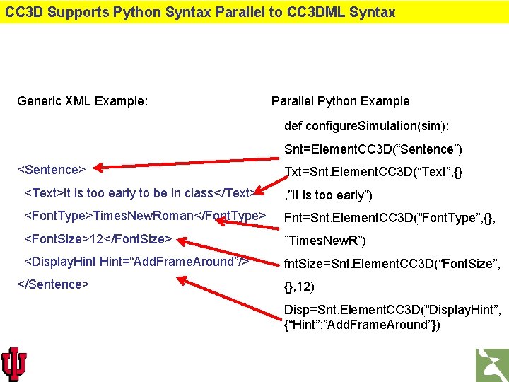
Generic XML 101 CC 3 DML is an XML, which stands for e. Xtensible Markup Language. A standard way to exchange information between different applications. XML Example: <Sentence> <Text>It is too early to be in class</Text> <Font. Type>Times. New. Roman</Font. Type> <Font. Size>12</Font. Size> <Display. Hint=“Add. Frame. Around”/> </Sentence>

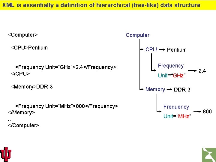
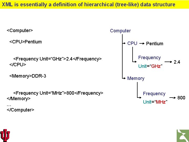
XML is essentially a definition of hierarchical (tree-like) data structure <Computer> <CPU>Pentium <Frequency Unit=“GHz”>2. 4</Frequency> </CPU> <Memory>DDR-3 <Frequency Unit=“MHz”>800</Frequency> </Memory> … </Computer> Computer CPU Pentium Frequency Unit=“GHz” Memory 2. 4 DDR-3 Frequency Unit=“MHz” 800

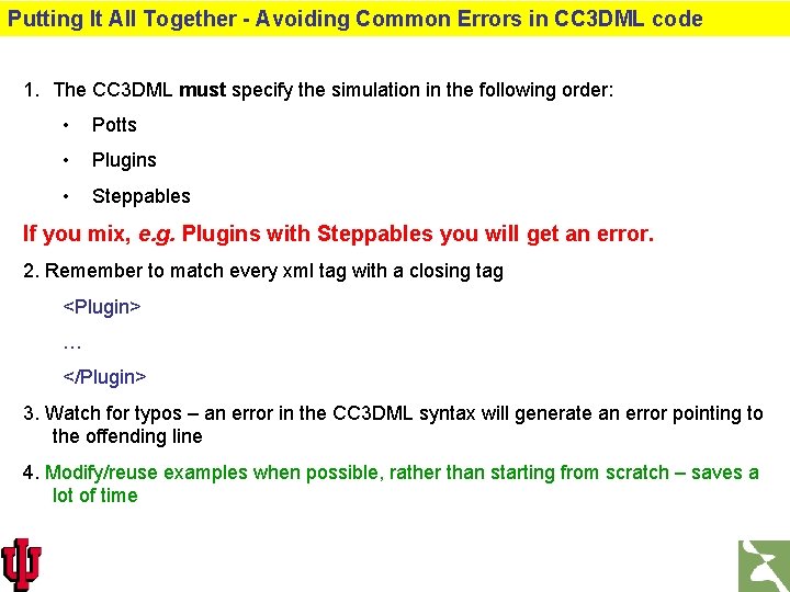
Putting It All Together - Avoiding Common Errors in CC 3 DML code 1. The CC 3 DML must specify the simulation in the following order: • Potts • Plugins • Steppables If you mix, e. g. Plugins with Steppables you will get an error. 2. Remember to match every xml tag with a closing tag <Plugin> … </Plugin> 3. Watch for typos – an error in the CC 3 DML syntax will generate an error pointing to the offending line 4. Modify/reuse examples when possible, rather than starting from scratch – saves a lot of time

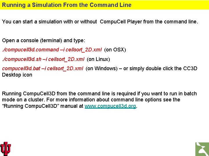
Running a Simulation From the Command Line You can start a simulation with or without Compu. Cell Player from the command line. Open a console (terminal) and type: . /compucell 3 d. command –i cellsort_2 D. xml (on OSX). /compucell 3 d. sh –i cellsort_2 D. xml (on Linux) compucell 3 d. bat –i cellsort_2 D. xml (on Windows) – or simply double click the CC 3 D Desktop icon Running Compu. Cell 3 D from the command line is required if you want to run in batch mode on a cluster. For more information about command line options see the “Running Compu. Cell 3 D” manual at www. compucell 3 d. org.

Cell-sorting simulation on square and hexagonal lattices The simulation parameters were kept the same for the two runs 1000 MCS

Replacing CC 3 DML with Python

CC 3 D Supports Python Syntax Parallel to CC 3 DML Syntax Generic XML Example: Parallel Python Example def configure. Simulation(sim): Snt=Element. CC 3 D(“Sentence”) <Sentence> Txt=Snt. Element. CC 3 D(“Text”, {} <Text>It is too early to be in class</Text> , ”It is too early”) <Font. Type>Times. New. Roman</Font. Type> Fnt=Snt. Element. CC 3 D(“Font. Type”, {}, <Font. Size>12</Font. Size> ”Times. New. R”) <Display. Hint=“Add. Frame. Around”/> fnt. Size=Snt. Element. CC 3 D(“Font. Size”, </Sentence> {}, 12) Disp=Snt. Element. CC 3 D(“Display. Hint”, {“Hint”: ”Add. Frame. Around”})

Choosing the Right Text Editor Since developing Compu. Cell 3 D simulation requires typing some simple code it is important that you have the right tools to do that most effectively. THE BEST EDITOR IS TWEDIT (supported by Consumer Research tests) • On Windows systems we also recommend Notepad++ editor: http: //notepad-plus. sourceforge. net/uk/site. htm • On Linux you have lots of choices: Kate (my favorite), gedit, mcedit etc. • On OSX situation you may use Smultron http: //sourceforge. net/projects/smultron/ or Text. Wrangler http: //www. barebones. com/products/textwrangler/ And as usual, if nothing else works there is always vi, emacs and punch-cards

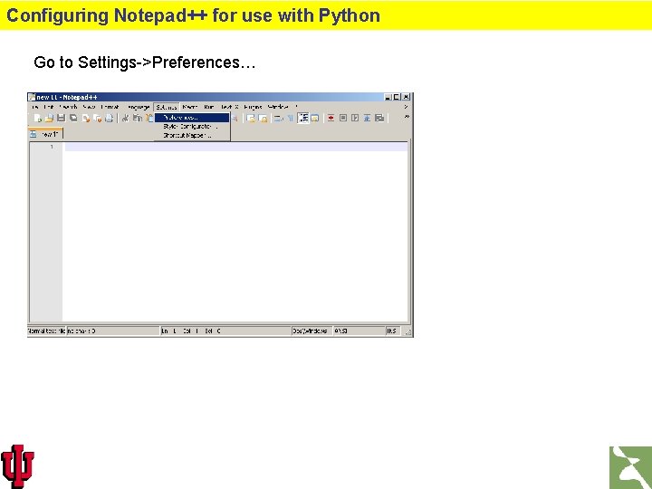
Configuring Notepad++ for use with Python Go to Settings->Preferences…

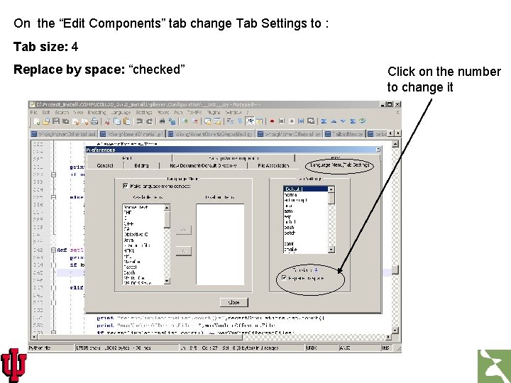
On the “Edit Components” tab change Tab Settings to : Tab size: 4 Replace by space: “checked” Click on the number to change it

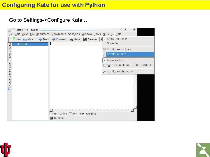
Configuring Kate for use with Python Go to Settings->Configure Kate …

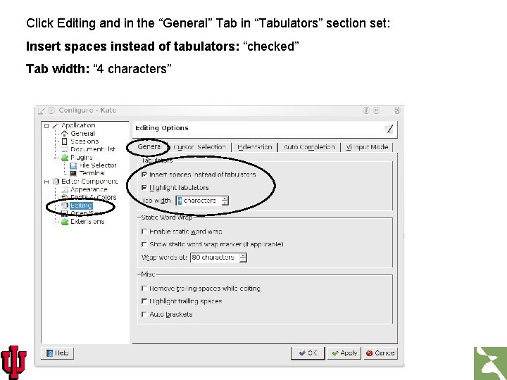
Click Editing and in the “General” Tab in “Tabulators” section set: Insert spaces instead of tabulators: “checked” Tab width: “ 4 characters”

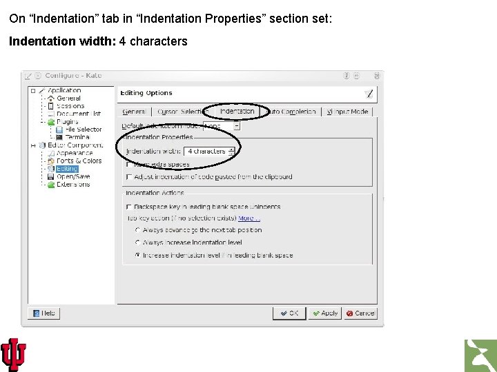
On “Indentation” tab in “Indentation Properties” section set: Indentation width: 4 characters

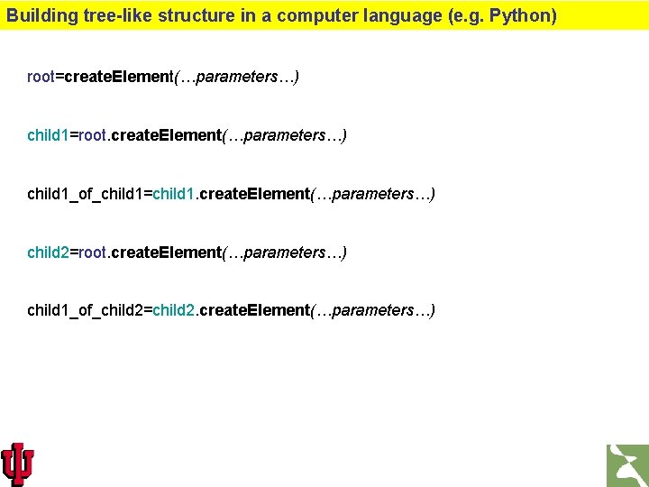
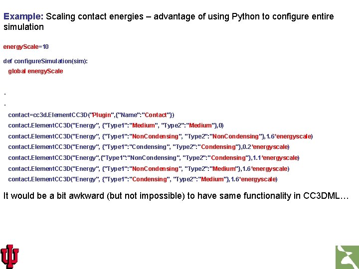
Using Python to describe entire simulations • Starting with 3. 2. 0 versions you may get rid of XML file and use Python to describe entire simulation. • The advantage of doing so is that you have one less file to worry about but also you may more easily manipulate simulation parameters. For example if you want contact energy between two cell types be twice as big as between two other cell types you could easily implement it in Python. Doing the same exercise with CC 3 DML is a bit harder (but not impossible). • Python syntax used to describe simulation closely mimics CC 3 DML syntax. There are however certain differences and inconsistencies caused by the fact that we are using different languages to accomplish same task. Currently there is no documentation explaining in detail Python syntax that replaces CC 3 DML. It will be developed soon • The most important reason for defining entire simulation in Python is the possibility of simulation steering i. e. the ability to dynamically change simulation parameters while simulation is running (available in 3. 2. 1) • The way you replace XML in Python is purely mechanical and we will show it on a simple example

XML is essentially a definition of hierarchical (tree-like) data structure <Computer> <CPU>Pentium <Frequency Unit=“GHz”>2. 4</Frequency> </CPU> <Memory>DDR-3 <Frequency Unit=“MHz”>800</Frequency> </Memory> … </Computer> Computer CPU Pentium Frequency Unit=“GHz” 2. 4 Memory Frequency Unit=“MHz” 800

Building tree-like structure in a computer language (e. g. Python) root=create. Element(…parameters…) child 1=root. create. Element(…parameters…) child 1_of_child 1=child 1. create. Element(…parameters…) child 2=root. create. Element(…parameters…) child 1_of_child 2=child 2. create. Element(…parameters…)

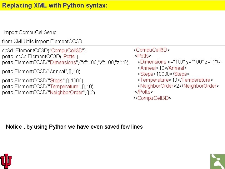
Replacing XML with Python syntax: import Compu. Cell. Setup from XMLUtils import Element. CC 3 D <Compu. Cell 3 D> cc 3 d=Element. CC 3 D("Compu. Cell 3 D") <Potts> potts=cc 3 d. Element. CC 3 D("Potts") <Dimensions x="100" y="100" z="1"/> potts. Element. CC 3 D("Dimensions", {"x": 100, "y": 100, "z": 1}) <Anneal>10</Anneal> potts. Element. CC 3 D(“Anneal”, {}, 10) <Steps>10000</Steps> <Temperature>10</Temperature> potts. Element. CC 3 D("Steps", {}, 1000) <Neighbor. Order>2</Neighbor. Order> potts. Element. CC 3 D("Temperature", {}, 10) </Potts> potts. Element. CC 3 D("Neighbor. Order", {}, 2) </Compu. Cell 3 D> Notice , by using Python we have even saved few lines

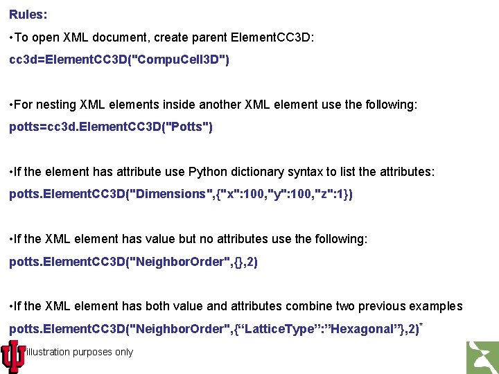
Rules: • To open XML document, create parent Element. CC 3 D: cc 3 d=Element. CC 3 D("Compu. Cell 3 D") • For nesting XML elements inside another XML element use the following: potts=cc 3 d. Element. CC 3 D("Potts") • If the element has attribute use Python dictionary syntax to list the attributes: potts. Element. CC 3 D("Dimensions", {"x": 100, "y": 100, "z": 1}) • If the XML element has value but no attributes use the following: potts. Element. CC 3 D("Neighbor. Order", {}, 2) • If the XML element has both value and attributes combine two previous examples potts. Element. CC 3 D("Neighbor. Order", {“Lattice. Type”: ”Hexagonal”}, 2)* *for illustration purposes only

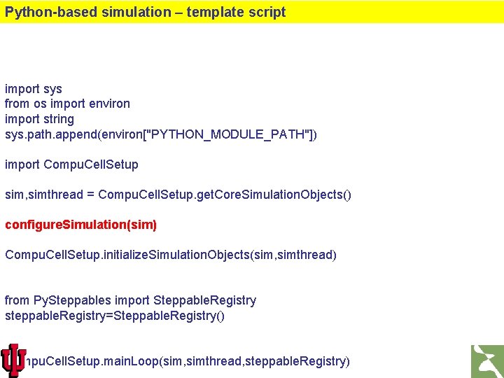
Python-based simulation – template script import sys from os import environ import string sys. path. append(environ["PYTHON_MODULE_PATH"]) import Compu. Cell. Setup sim, simthread = Compu. Cell. Setup. get. Core. Simulation. Objects() configure. Simulation(sim) Compu. Cell. Setup. initialize. Simulation. Objects(sim, simthread) from Py. Steppables import Steppable. Registry steppable. Registry=Steppable. Registry() Compu. Cell. Setup. main. Loop(sim, simthread, steppable. Registry)

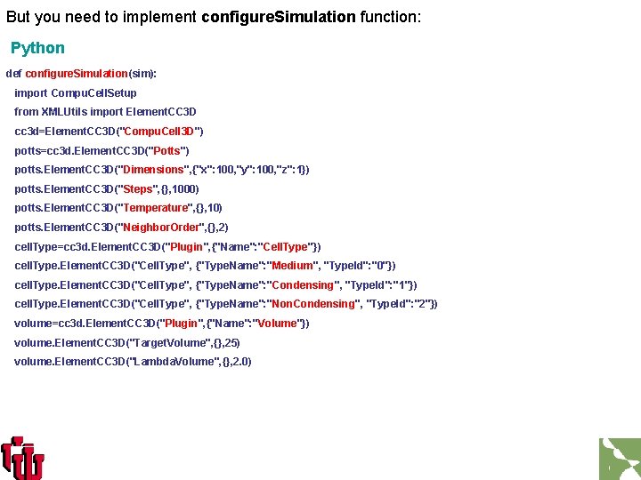
But you need to implement configure. Simulation function: Python def configure. Simulation(sim): import Compu. Cell. Setup from XMLUtils import Element. CC 3 D cc 3 d=Element. CC 3 D("Compu. Cell 3 D") potts=cc 3 d. Element. CC 3 D("Potts") potts. Element. CC 3 D("Dimensions", {"x": 100, "y": 100, "z": 1}) potts. Element. CC 3 D("Steps", {}, 1000) potts. Element. CC 3 D("Temperature", {}, 10) potts. Element. CC 3 D("Neighbor. Order", {}, 2) cell. Type=cc 3 d. Element. CC 3 D("Plugin", {"Name": "Cell. Type"}) cell. Type. Element. CC 3 D("Cell. Type", {"Type. Name": "Medium", "Type. Id": "0"}) cell. Type. Element. CC 3 D("Cell. Type", {"Type. Name": "Condensing", "Type. Id": "1"}) cell. Type. Element. CC 3 D("Cell. Type", {"Type. Name": "Non. Condensing", "Type. Id": "2"}) volume=cc 3 d. Element. CC 3 D("Plugin", {"Name": "Volume"}) volume. Element. CC 3 D("Target. Volume", {}, 25) volume. Element. CC 3 D("Lambda. Volume", {}, 2. 0)

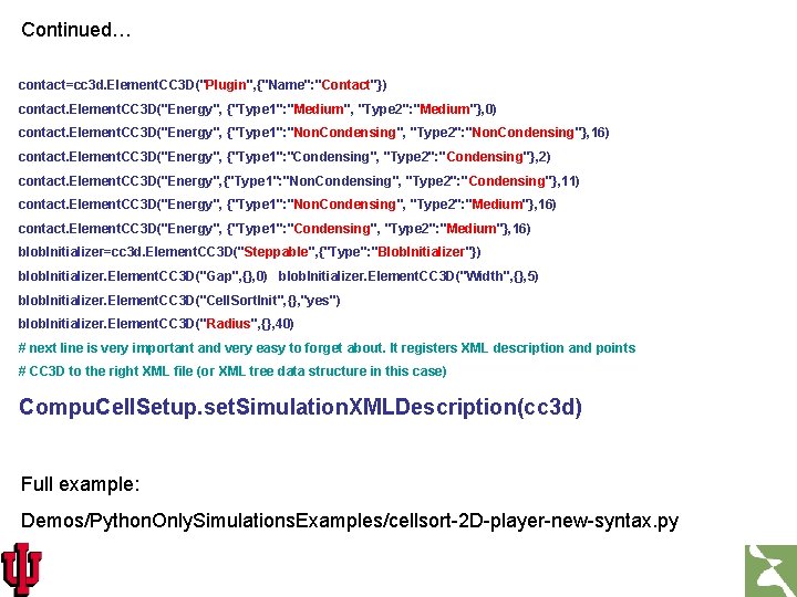
Continued… contact=cc 3 d. Element. CC 3 D("Plugin", {"Name": "Contact"}) contact. Element. CC 3 D("Energy", {"Type 1": "Medium", "Type 2": "Medium"}, 0) contact. Element. CC 3 D("Energy", {"Type 1": "Non. Condensing", "Type 2": "Non. Condensing"}, 16) contact. Element. CC 3 D("Energy", {"Type 1": "Condensing", "Type 2": "Condensing"}, 2) contact. Element. CC 3 D("Energy", {"Type 1": "Non. Condensing", "Type 2": "Condensing"}, 11) contact. Element. CC 3 D("Energy", {"Type 1": "Non. Condensing", "Type 2": "Medium"}, 16) contact. Element. CC 3 D("Energy", {"Type 1": "Condensing", "Type 2": "Medium"}, 16) blob. Initializer=cc 3 d. Element. CC 3 D("Steppable", {"Type": "Blob. Initializer"}) blob. Initializer. Element. CC 3 D("Gap", {}, 0) blob. Initializer. Element. CC 3 D("Width", {}, 5) blob. Initializer. Element. CC 3 D("Cell. Sort. Init", {}, "yes") blob. Initializer. Element. CC 3 D("Radius", {}, 40) # next line is very important and very easy to forget about. It registers XML description and points # CC 3 D to the right XML file (or XML tree data structure in this case) Compu. Cell. Setup. set. Simulation. XMLDescription(cc 3 d) Full example: Demos/Python. Only. Simulations. Examples/cellsort-2 D-player-new-syntax. py

Example: Scaling contact energies – advantage of using Python to configure entire simulation energy. Scale=10 def configure. Simulation(sim): global energy. Scale . . contact=cc 3 d. Element. CC 3 D("Plugin", {"Name": "Contact"}) contact. Element. CC 3 D("Energy", {"Type 1": "Medium", "Type 2": "Medium"}, 0) contact. Element. CC 3 D("Energy", {"Type 1": "Non. Condensing", "Type 2": "Non. Condensing"}, 1. 6*energyscale) contact. Element. CC 3 D("Energy", {"Type 1": "Condensing", "Type 2": "Condensing"}, 0. 2*energyscale) contact. Element. CC 3 D("Energy", {"Type 1": "Non. Condensing", "Type 2": "Condensing"}, 1. 1*energyscale) contact. Element. CC 3 D("Energy", {"Type 1": "Non. Condensing", "Type 2": "Medium"}, 1. 6*energyscale) contact. Element. CC 3 D("Energy", {"Type 1": "Condensing", "Type 2": "Medium"}, 1. 6*energyscale) It would be a bit awkward (but not impossible) to have same functionality in CC 3 DML…

Major Plugins and Steppables Available in Compu. Cell 3 D

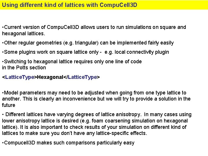
Using different kind of lattices with Compu. Cell 3 D • Current version of Compu. Cell 3 D allows users to run simulations on square and hexagonal lattices. • Other regular geometries (e. g. triangular) can be implemented fairly easily • Some plugins work on square lattice only - e. g. local connectivity plugin • Switching to hexagonal lattice requires only one line of code in the Potts section <Lattice. Type>Hexagonal</Lattice. Type> • Model parameters may need to be adjusted when going from one type lattice to another. This is clearly an inconvenience but we will try to provide a solution in the future • Different lattices have varying degrees of lattice anisotropy. In many cases using lower anisotropy lattice is desired (e. g. foam coarsening simulation on hexagonal lattice). It is also important to check results of your simulation on different kind of lattices to make sure you don’t have any lattice-specific effects. • Compucell 3 D makes such comparisons particularly easy

Nearest neighbors in 2 D and their Euclidian distances from the central pixel 4 4 3 2 3 1 4 2 1 2 4 3 2 4 1 1 2 3 4 4 3 2 2 4 2 3 4 2 D Square Lattice 1 1 3 4 2 1 1 4 4 3 2 4 4 3 4 2 D Hexagonal Lattice Square. Lattice: Neighbo r Order Number of Neighbors Euclidian Distance Number of Neighbors 1 4 1 6 2 4 3 4 4 8 2 Euclidian Distance Square in 2 D Cube in 3 D 6 Hexagonal lattice: 6 Hexagon in 2 D 12 Rhombic dodecahedron in 3 D

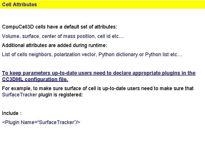
Cell Attributes Compu. Cell 3 D cells have a default set of attributes: Volume, surface, center of mass position, cell id etc… Additional attributes are added during runtime: List of cells neighbors, polarization vector, Python dictionary or Python list etc… To keep parameters up-to-date users need to declare appropriate plugins in the CC 3 DML configuration file. For example, to make surface of cell is up-to-date users need to make sure that Surface. Tracker plugin is registered: Include : <Plugin Name=“Surface. Tracker”/>

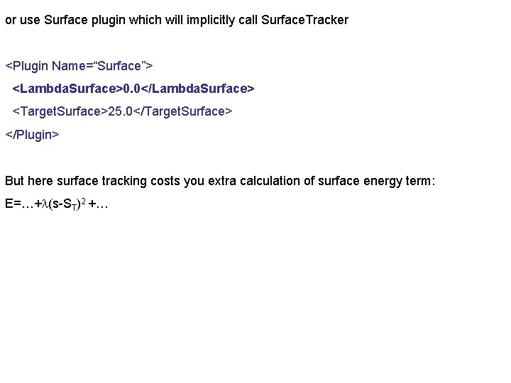
or use Surface plugin which will implicitly call Surface. Tracker <Plugin Name=“Surface”> <Lambda. Surface>0. 0</Lambda. Surface> <Target. Surface>25. 0</Target. Surface> </Plugin> But here surface tracking costs you extra calculation of surface energy term: E=…+l(s-ST)2 +…

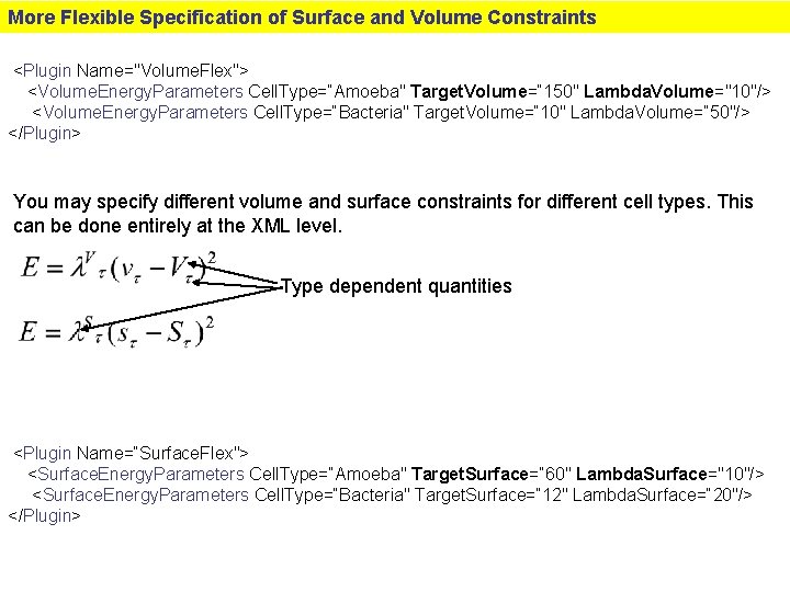
More Flexible Specification of Surface and Volume Constraints <Plugin Name="Volume. Flex"> <Volume. Energy. Parameters Cell. Type=“Amoeba" Target. Volume=“ 150" Lambda. Volume="10"/> <Volume. Energy. Parameters Cell. Type=“Bacteria" Target. Volume=“ 10" Lambda. Volume=“ 50"/> </Plugin> You may specify different volume and surface constraints for different cell types. This can be done entirely at the XML level. Type dependent quantities <Plugin Name=“Surface. Flex"> <Surface. Energy. Parameters Cell. Type=“Amoeba" Target. Surface=“ 60" Lambda. Surface="10"/> <Surface. Energy. Parameters Cell. Type=“Bacteria" Target. Surface=“ 12" Lambda. Surface=“ 20"/> </Plugin>

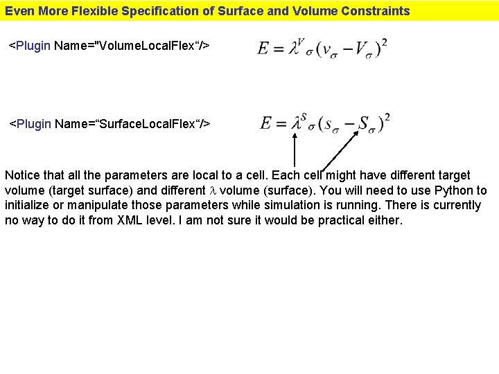
Even More Flexible Specification of Surface and Volume Constraints <Plugin Name="Volume. Local. Flex“/> <Plugin Name=“Surface. Local. Flex“/> Notice that all the parameters are local to a cell. Each cell might have different target volume (target surface) and different l volume (surface). You will need to use Python to initialize or manipulate those parameters while simulation is running. There is currently no way to do it from XML level. I am not sure it would be practical either.

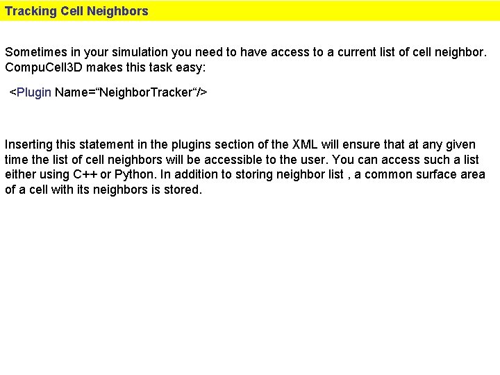
Tracking Cell Neighbors Sometimes in your simulation you need to have access to a current list of cell neighbor. Compu. Cell 3 D makes this task easy: <Plugin Name=“Neighbor. Tracker“/> Inserting this statement in the plugins section of the XML will ensure that at any given time the list of cell neighbors will be accessible to the user. You can access such a list either using C++ or Python. In addition to storing neighbor list , a common surface area of a cell with its neighbors is stored.

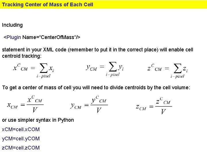
Tracking Center of Mass of Each Cell Including <Plugin Name=“Center. Of. Mass“/> statement in your XML code (remember to put it in the correct place) will enable cell centroid tracking: To get a center of mass of cell you will need to divide centroids by the cell volume: or use simpler syntax in Python x. CM=cell. x. COM y. CM=cell. y. COM z. CM=cell. z. COM

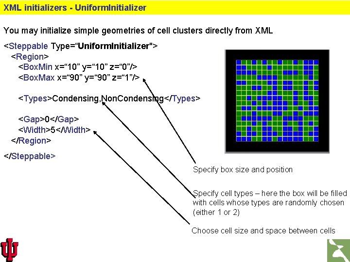
XML initializers - Uniform. Initializer You may initialize simple geometries of cell clusters directly from XML <Steppable Type=“Uniform. Initializer"> <Region> <Box. Min x=“ 10” y=“ 10” z=“ 0”/> <Box. Max x=“ 90” y=“ 90” z=“ 1”/> <Types>Condensing, Non. Condensing</Types> <Gap>0</Gap> <Width>5</Width> </Region> </Steppable> Specify box size and position Specify cell types – here the box will be filled with cells whose types are randomly chosen (either 1 or 2) Choose cell size and space between cells

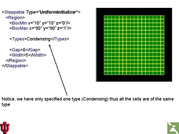
<Steppable Type=“Uniform. Initializer"> <Region> <Box. Min x=“ 10” y=“ 10” z=“ 0”/> <Box. Max x=“ 90” y=“ 90” z=“ 1”/> <Types>Condensing</Types> <Gap>0</Gap> <Width>5</Width> </Region> </Steppable> Notice, we have only specified one type (Condensing) thus all the cells are of the same type

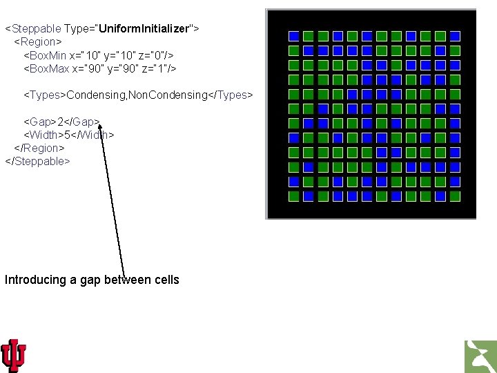
<Steppable Type=“Uniform. Initializer"> <Region> <Box. Min x=“ 10” y=“ 10” z=“ 0”/> <Box. Max x=“ 90” y=“ 90” z=“ 1”/> <Types>Condensing, Non. Condensing</Types> <Gap>2</Gap> <Width>5</Width> </Region> </Steppable> Introducing a gap between cells

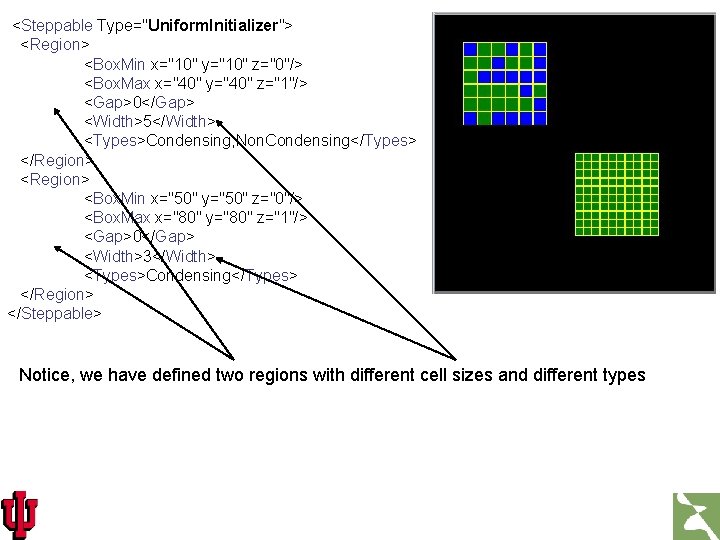
<Steppable Type="Uniform. Initializer"> <Region> <Box. Min x="10" y="10" z="0"/> <Box. Max x="40" y="40" z="1"/> <Gap>0</Gap> <Width>5</Width> <Types>Condensing, Non. Condensing</Types> </Region> <Box. Min x="50" y="50" z="0"/> <Box. Max x="80" y="80" z="1"/> <Gap>0</Gap> <Width>3</Width> <Types>Condensing</Types> </Region> </Steppable> Notice, we have defined two regions with different cell sizes and different types

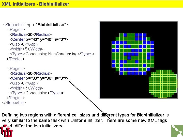
XML initializers - Blob. Initializer <Steppable Type="Blob. Initializer"> <Region> <Radius>30</Radius> <Center x="40" y="40" z="0"/> <Gap>0</Gap> <Width>5</Width> <Types>Condensing, Non. Condensing</Types> </Region> <Radius>20</Radius> <Center x="80" y="80" z="0"/> <Gap>0</Gap> <Width>3</Width> <Types>Condensing</Types> </Region> </Steppable> Defining two regions with different cell sizes and different types for Blob. Initializer is very similar to the same task with Uniform. Initilizer. There are some new XML tags which differ the two initializers.

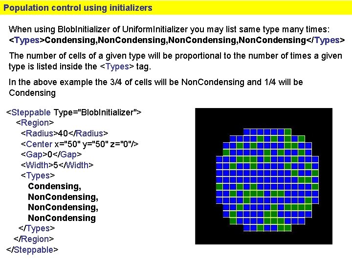
Population control using initializers When using Blob. Initializer of Uniform. Initializer you may list same type many times: <Types>Condensing, Non. Condensing</Types> The number of cells of a given type will be proportional to the number of times a given type is listed inside the <Types> tag. In the above example the 3/4 of cells will be Non. Condensing and 1/4 will be Condensing <Steppable Type="Blob. Initializer"> <Region> <Radius>40</Radius> <Center x="50" y="50" z="0"/> <Gap>0</Gap> <Width>5</Width> <Types> Condensing, Non. Condensing </Types> </Region> </Steppable>

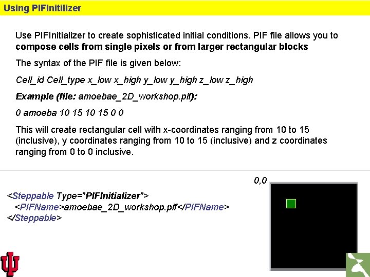
Using PIFInitilizer Use PIFInitializer to create sophisticated initial conditions. PIF file allows you to compose cells from single pixels or from larger rectangular blocks The syntax of the PIF file is given below: Cell_id Cell_type x_low x_high y_low y_high z_low z_high Example (file: amoebae_2 D_workshop. pif): 0 amoeba 10 15 0 0 This will create rectangular cell with x-coordinates ranging from 10 to 15 (inclusive), y coordinates ranging from 10 to 15 (inclusive) and z coordinates ranging from 0 to 0 inclusive. 0, 0 <Steppable Type="PIFInitializer"> <PIFName>amoebae_2 D_workshop. pif</PIFName> </Steppable>

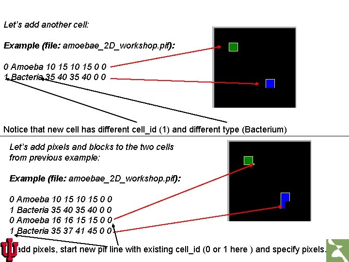
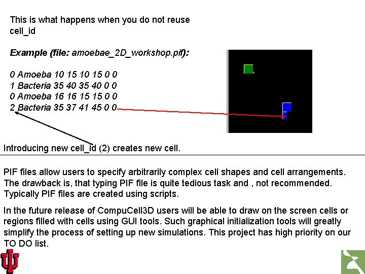
Let’s add another cell: Example (file: amoebae_2 D_workshop. pif): 0 Amoeba 10 15 0 0 1 Bacteria 35 40 0 0 Notice that new cell has different cell_id (1) and different type (Bacterium) Let’s add pixels and blocks to the two cells from previous example: Example (file: amoebae_2 D_workshop. pif): 0 Amoeba 10 15 0 0 1 Bacteria 35 40 0 0 0 Amoeba 16 16 15 15 0 0 1 Bacteria 35 37 41 45 0 0 To add pixels, start new pif line with existing cell_id (0 or 1 here ) and specify pixels.

This is what happens when you do not reuse cell_id Example (file: amoebae_2 D_workshop. pif): 0 Amoeba 10 15 0 0 1 Bacteria 35 40 0 0 0 Amoeba 16 16 15 15 0 0 2 Bacteria 35 37 41 45 0 0 Introducing new cell_id (2) creates new cell. PIF files allow users to specify arbitrarily complex cell shapes and cell arrangements. The drawback is, that typing PIF file is quite tedious task and , not recommended. Typically PIF files are created using scripts. In the future release of Compu. Cell 3 D users will be able to draw on the screen cells or regions filled with cells using GUI tools. Such graphical initialization tools will greatly simplify the process of setting up new simulations. This project has high priority on our TO DO list.

PIFDumper - yet another way to create initial condition PIFDumper is typically used to output cell lattice every predefined number of MCS. It is useful because, you may start with rectangular cells, “round them up” by running Compu. Cell 3 D , output cell lattice using PIF dumper and reload newly created PIF file using PIFInitializer. <Steppable Type="PIFDumper“ Frequency=“ 100”> <PIFName>amoebae</PIFName> </Steppable> Above syntax tells Compu. Cell 3 D to store cell lattice as a PIF file every 100 MCS. The files will be named amoebae. 100. pif , amoebae. 200. pif etc… To reload file , say amoebae. 100. pif use already familiar syntax: <Steppable Type="PIFInitializer"> <PIFName>amoebae. 100. pif</PIFName> </Steppable>

PIFTracer and other PIF Generators See presentation by Mitja Hmeljak

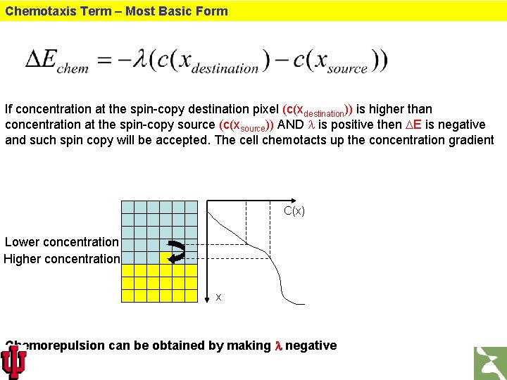
Chemotaxis Basic facts • Chemotaxis is defined as cell motion induced by a presence (gradient) of a chemical. • In GGH formalism chemotaxis is implemented as a spin copy bias which depends on chemical gradient. • Chemotaxis was first introduced to GGH formalism by Paulien Hogeweg from University of Utrecht, Netherlands • In Compu. Cell 3 D Chemotaxis plugin provides wide range of options to support different modes of chemotaxis. • Chemotaxis plugin requires the presence of at least one concentration field. The fields can be inserted into Compu. Cell 3 D simulation by means PDE solvers or can be created, initialized and managed explicitly from the Python level

Chemotaxis Term – Most Basic Form If concentration at the spin-copy destination pixel (c(xdestination)) is higher than concentration at the spin-copy source (c(xsource)) AND l is positive then DE is negative and such spin copy will be accepted. The cell chemotacts up the concentration gradient C(x) Lower concentration Higher concentration x Chemorepulsion can be obtained by making l negative

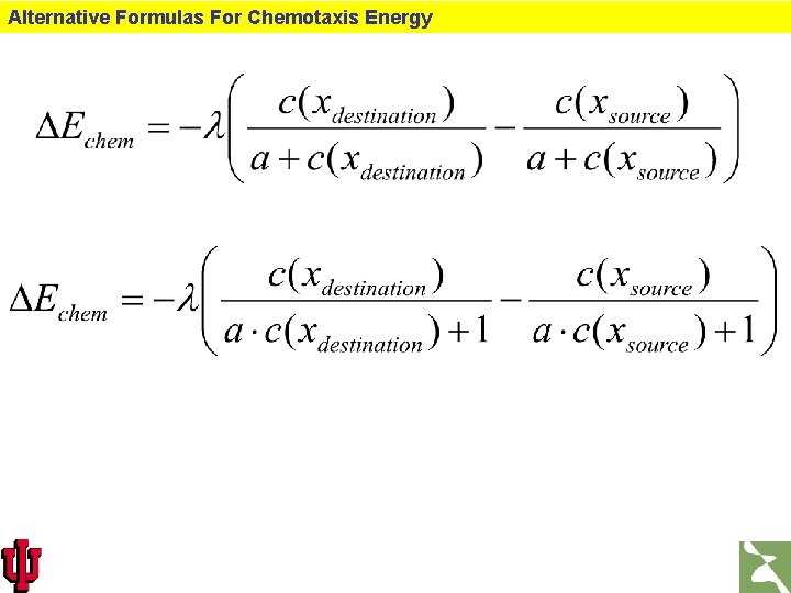
Alternative Formulas For Chemotaxis Energy

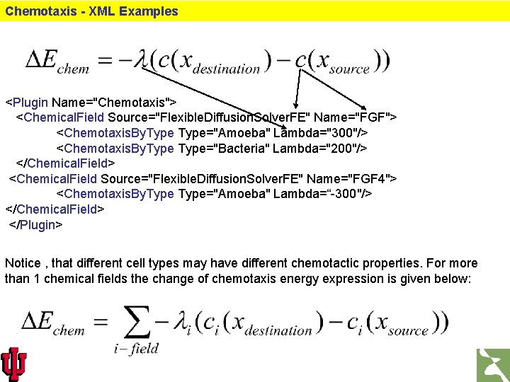
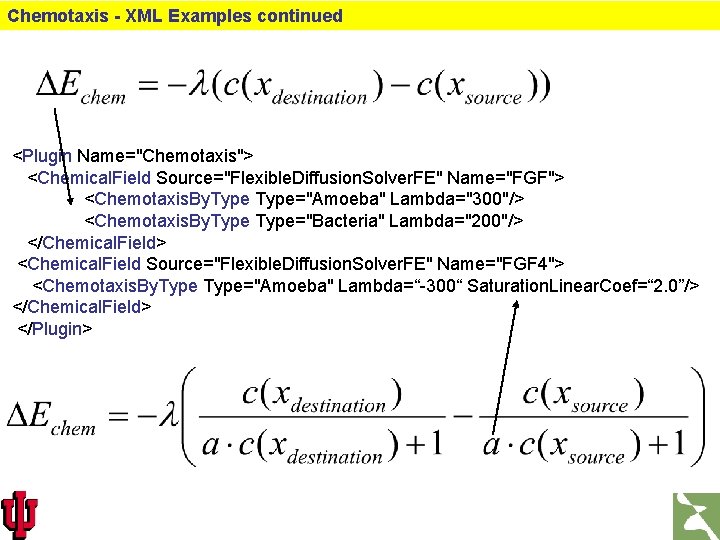
Chemotaxis - XML Examples <Plugin Name="Chemotaxis"> <Chemical. Field Source="Flexible. Diffusion. Solver. FE" Name="FGF"> <Chemotaxis. By. Type="Amoeba" Lambda="300"/> <Chemotaxis. By. Type="Bacteria" Lambda="200"/> </Chemical. Field> <Chemical. Field Source="Flexible. Diffusion. Solver. FE" Name="FGF 4"> <Chemotaxis. By. Type="Amoeba" Lambda=“-300"/> </Chemical. Field> </Plugin> Notice , that different cell types may have different chemotactic properties. For more than 1 chemical fields the change of chemotaxis energy expression is given below:

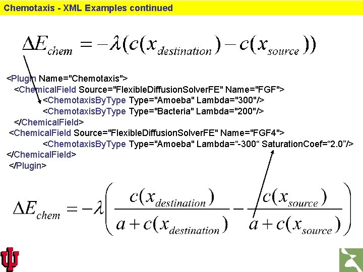
Chemotaxis - XML Examples continued <Plugin Name="Chemotaxis"> <Chemical. Field Source="Flexible. Diffusion. Solver. FE" Name="FGF"> <Chemotaxis. By. Type="Amoeba" Lambda="300"/> <Chemotaxis. By. Type="Bacteria" Lambda="200"/> </Chemical. Field> <Chemical. Field Source="Flexible. Diffusion. Solver. FE" Name="FGF 4"> <Chemotaxis. By. Type="Amoeba" Lambda=“-300“ Saturation. Coef=“ 2. 0”/> </Chemical. Field> </Plugin>

Chemotaxis - XML Examples continued <Plugin Name="Chemotaxis"> <Chemical. Field Source="Flexible. Diffusion. Solver. FE" Name="FGF"> <Chemotaxis. By. Type="Amoeba" Lambda="300"/> <Chemotaxis. By. Type="Bacteria" Lambda="200"/> </Chemical. Field> <Chemical. Field Source="Flexible. Diffusion. Solver. FE" Name="FGF 4"> <Chemotaxis. By. Type="Amoeba" Lambda=“-300“ Saturation. Linear. Coef=“ 2. 0”/> </Chemical. Field> </Plugin>

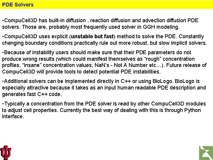
PDE Solvers • Compu. Cell 3 D has built-in diffusion , reaction diffusion and advection diffusion PDE solvers. Those are, probably most frequently used solver in GGH modeling. • Compu. Cell 3 D uses explicit (unstable but fast) method to solve the PDE. Constantly changing boundary conditions practically rule out more robust, but slow implicit solvers. • Because of instability users should make sure that their PDE parameters do not produce wrong results (which could manifest themselves as “rough” concentration profiles, “insane” concentration values, Na. N’s - Not A Number etc…). Future release of Compu. Cell 3 D will provide tools to detect potential PDE instabilities. • Additional solvers can be implemented directly in C++ or using Bio. Logo is especially attractive because it takes as an input human readable PDE description and generates fast C++ code. • Typically a concentration from the PDE solver is read by other Compu. Cell 3 D modules to adjust cell properties. Currently the best way of dealing with this is through Python interface.

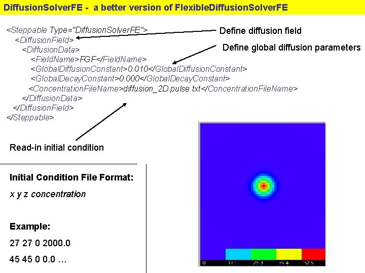
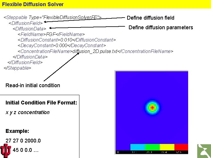
Diffusion. Solver. FE - a better version of Flexible. Diffusion. Solver. FE <Steppable Type="Diffusion. Solver. FE"> Define diffusion field <Diffusion. Field> Define global diffusion parameters <Diffusion. Data> <Field. Name>FGF</Field. Name> <Global. Diffusion. Constant>0. 010</Global. Diffusion. Constant> <Global. Decay. Constant>0. 000</Global. Decay. Constant> <Concentration. File. Name>diffusion_2 D. pulse. txt</Concentration. File. Name> </Diffusion. Data> </Diffusion. Field> </Steppable> Read-in initial condition Initial Condition File Format: x y z concentration Example: 27 27 0 2000. 0 45 45 0 0. 0 …

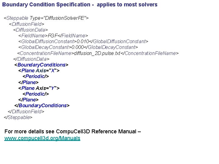
Boundary Condition Specification - applies to most solvers <Steppable Type="Diffusion. Solver. FE"> <Diffusion. Field> <Diffusion. Data> <Field. Name>FGF</Field. Name> <Global. Diffusion. Constant>0. 010</Global. Diffusion. Constant> <Global. Decay. Constant>0. 000</Global. Decay. Constant> <Concentration. File. Name>diffusion_2 D. pulse. txt</Concentration. File. Name> </Diffusion. Data> <Boundary. Conditions> <Plane Axis="X"> <Periodic/> </Plane> <Plane Axis="Y"> <Periodic/> </Plane> </Boundary. Conditions> </Diffusion. Field> </Steppable> For more details see Compu. Cell 3 D Reference Manual – www. compucell 3 d. org/Manuals

Flexible Diffusion Solver <Steppable Type="Flexible. Diffusion. Solver. FE"> Define diffusion field <Diffusion. Field> Define diffusion parameters <Diffusion. Data> <Field. Name>FGF</Field. Name> <Diffusion. Constant>0. 010</Diffusion. Constant> <Decay. Constant>0. 000</Decay. Constant> <Concentration. File. Name>diffusion_2 D. pulse. txt</Concentration. File. Name> </Diffusion. Data> </Diffusion. Field> </Steppable> Read-in initial condition Initial Condition File Format: x y z concentration Example: 27 27 0 2000. 0 45 45 0 0. 0 …

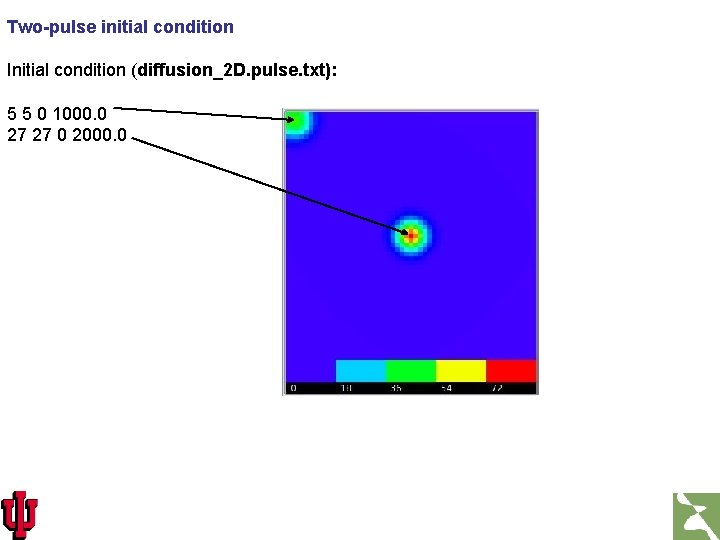
Two-pulse initial condition Initial condition (diffusion_2 D. pulse. txt): 5 5 0 1000. 0 27 27 0 2000. 0

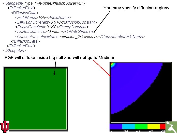
<Steppable Type="Flexible. Diffusion. Solver. FE"> <Diffusion. Field> You may specify diffusion regions <Diffusion. Data> <Field. Name>FGF</Field. Name> <Diffusion. Constant>0. 010</Diffusion. Constant> <Decay. Constant>0. 000</Decay. Constant> <Do. Not. Diffuse. To>Medium</Do. Not. Diffuse. To> <Concentration. File. Name>diffusion_2 D. pulse. txt</Concentration. File. Name> </Diffusion. Data> </Diffusion. Field> </Steppable> FGF will diffuse inside big cell and will not go to Medium

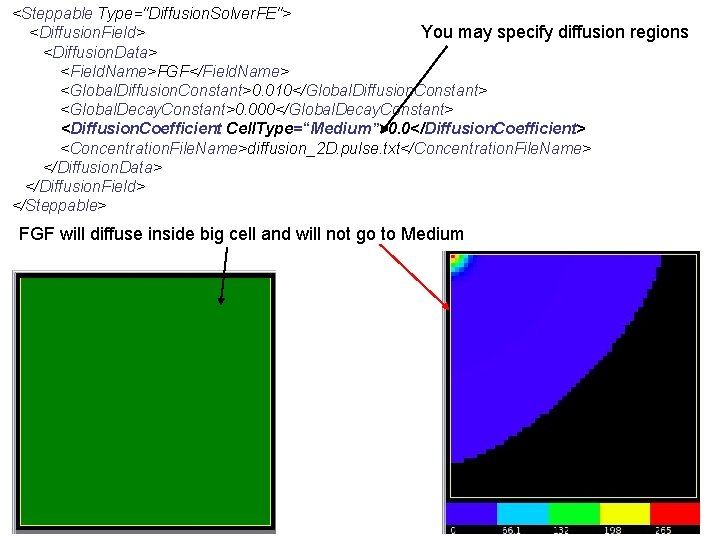
<Steppable Type="Diffusion. Solver. FE"> <Diffusion. Field> You may specify diffusion regions <Diffusion. Data> <Field. Name>FGF</Field. Name> <Global. Diffusion. Constant>0. 010</Global. Diffusion. Constant> <Global. Decay. Constant>0. 000</Global. Decay. Constant> <Diffusion. Coefficient Cell. Type=“Medium”>0. 0</Diffusion. Coefficient> <Concentration. File. Name>diffusion_2 D. pulse. txt</Concentration. File. Name> </Diffusion. Data> </Diffusion. Field> </Steppable> FGF will diffuse inside big cell and will not go to Medium

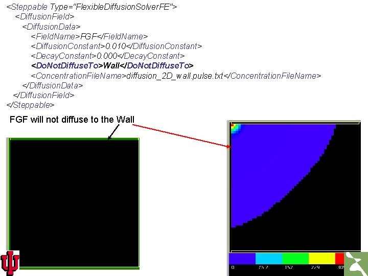
<Steppable Type="Flexible. Diffusion. Solver. FE"> <Diffusion. Field> <Diffusion. Data> <Field. Name>FGF</Field. Name> <Diffusion. Constant>0. 010</Diffusion. Constant> <Decay. Constant>0. 000</Decay. Constant> <Do. Not. Diffuse. To>Wall</Do. Not. Diffuse. To> <Concentration. File. Name>diffusion_2 D_wall. pulse. txt</Concentration. File. Name> </Diffusion. Data> </Diffusion. Field> </Steppable> FGF will not diffuse to the Wall

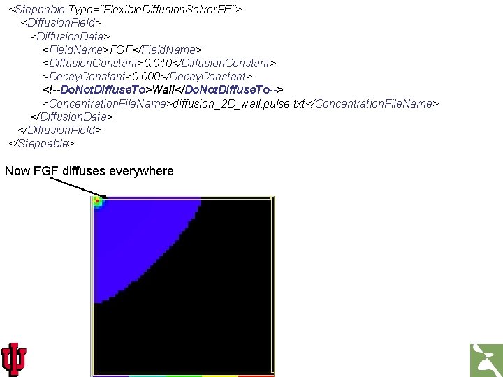
<Steppable Type="Flexible. Diffusion. Solver. FE"> <Diffusion. Field> <Diffusion. Data> <Field. Name>FGF</Field. Name> <Diffusion. Constant>0. 010</Diffusion. Constant> <Decay. Constant>0. 000</Decay. Constant> <!--Do. Not. Diffuse. To>Wall</Do. Not. Diffuse. To--> <Concentration. File. Name>diffusion_2 D_wall. pulse. txt</Concentration. File. Name> </Diffusion. Data> </Diffusion. Field> </Steppable> Now FGF diffuses everywhere

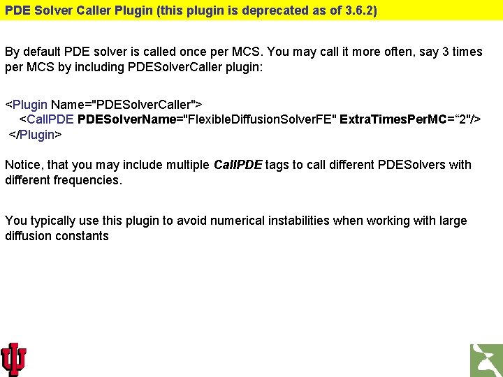
PDE Solver Caller Plugin (this plugin is deprecated as of 3. 6. 2) By default PDE solver is called once per MCS. You may call it more often, say 3 times per MCS by including PDESolver. Caller plugin: <Plugin Name="PDESolver. Caller"> <Call. PDESolver. Name="Flexible. Diffusion. Solver. FE" Extra. Times. Per. MC=“ 2"/> </Plugin> Notice, that you may include multiple Call. PDE tags to call different PDESolvers with different frequencies. You typically use this plugin to avoid numerical instabilities when working with large diffusion constants

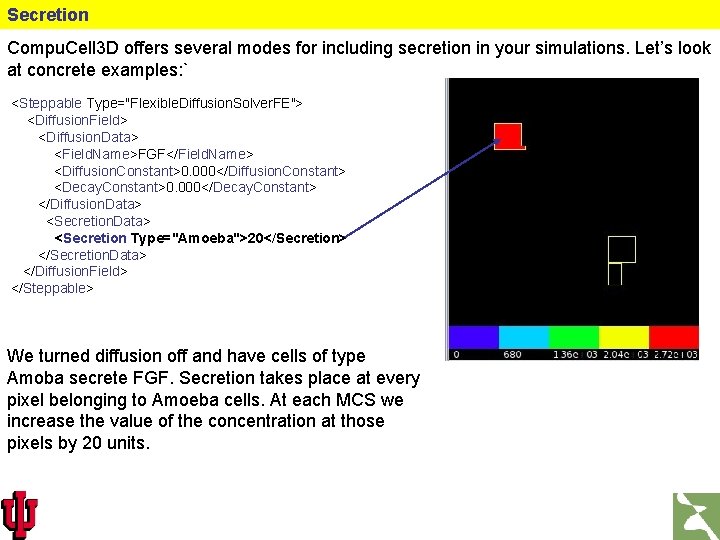
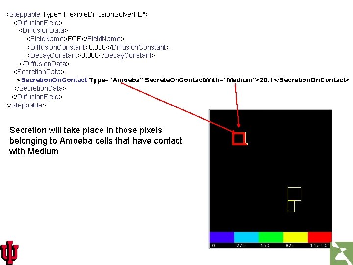
Secretion Compu. Cell 3 D offers several modes for including secretion in your simulations. Let’s look at concrete examples: ` <Steppable Type="Flexible. Diffusion. Solver. FE"> <Diffusion. Field> <Diffusion. Data> <Field. Name>FGF</Field. Name> <Diffusion. Constant>0. 000</Diffusion. Constant> <Decay. Constant>0. 000</Decay. Constant> </Diffusion. Data> <Secretion Type="Amoeba">20</Secretion> </Secretion. Data> </Diffusion. Field> </Steppable> We turned diffusion off and have cells of type Amoba secrete FGF. Secretion takes place at every pixel belonging to Amoeba cells. At each MCS we increase the value of the concentration at those pixels by 20 units.

<Steppable Type="Flexible. Diffusion. Solver. FE"> <Diffusion. Field> <Diffusion. Data> <Field. Name>FGF</Field. Name> <Diffusion. Constant>0. 000</Diffusion. Constant> <Decay. Constant>0. 000</Decay. Constant> </Diffusion. Data> <Secretion. On. Contact Type=“Amoeba" Secrete. On. Contact. With=“Medium">20. 1</Secretion. On. Contact> </Secretion. Data> </Diffusion. Field> </Steppable> Secretion will take place in those pixels belonging to Amoeba cells that have contact with Medium

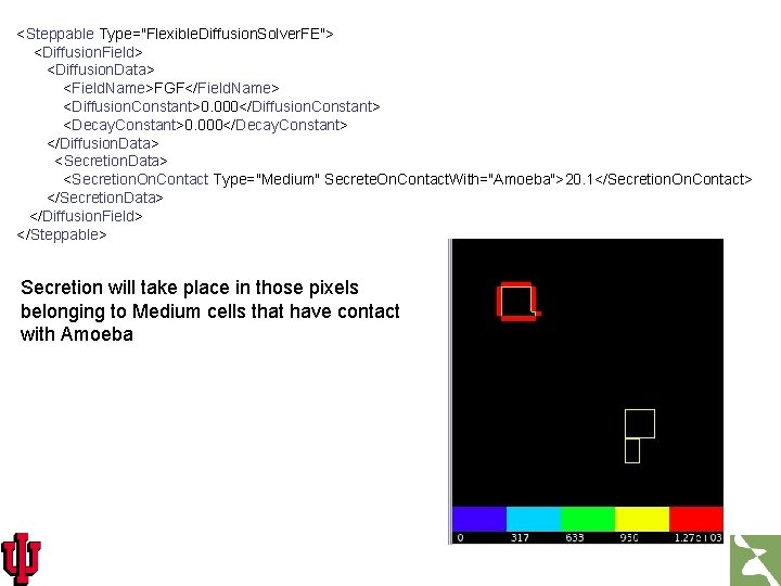
<Steppable Type="Flexible. Diffusion. Solver. FE"> <Diffusion. Field> <Diffusion. Data> <Field. Name>FGF</Field. Name> <Diffusion. Constant>0. 000</Diffusion. Constant> <Decay. Constant>0. 000</Decay. Constant> </Diffusion. Data> <Secretion. On. Contact Type="Medium" Secrete. On. Contact. With="Amoeba">20. 1</Secretion. On. Contact> </Secretion. Data> </Diffusion. Field> </Steppable> Secretion will take place in those pixels belonging to Medium cells that have contact with Amoeba

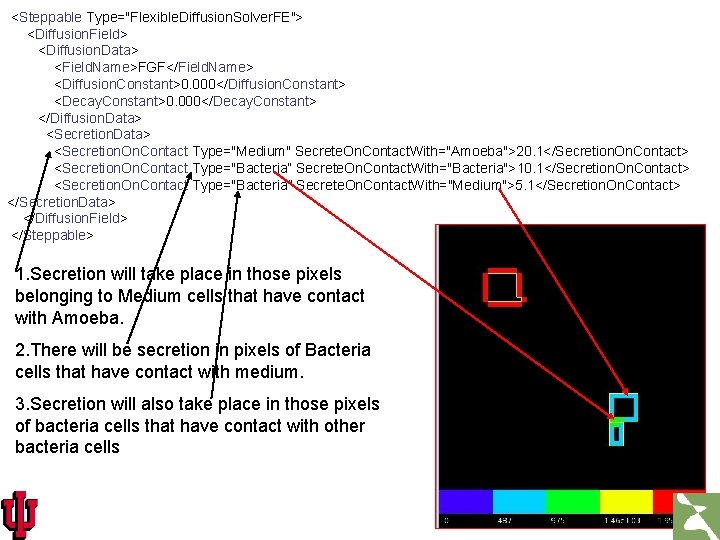
<Steppable Type="Flexible. Diffusion. Solver. FE"> <Diffusion. Field> <Diffusion. Data> <Field. Name>FGF</Field. Name> <Diffusion. Constant>0. 000</Diffusion. Constant> <Decay. Constant>0. 000</Decay. Constant> </Diffusion. Data> <Secretion. On. Contact Type="Medium" Secrete. On. Contact. With="Amoeba">20. 1</Secretion. On. Contact> <Secretion. On. Contact Type="Bacteria“ Secrete. On. Contact. With="Bacteria">10. 1</Secretion. On. Contact> <Secretion. On. Contact Type="Bacteria" Secrete. On. Contact. With="Medium">5. 1</Secretion. On. Contact> </Secretion. Data> </Diffusion. Field> </Steppable> 1. Secretion will take place in those pixels belonging to Medium cells that have contact with Amoeba. 2. There will be secretion in pixels of Bacteria cells that have contact with medium. 3. Secretion will also take place in those pixels of bacteria cells that have contact with other bacteria cells

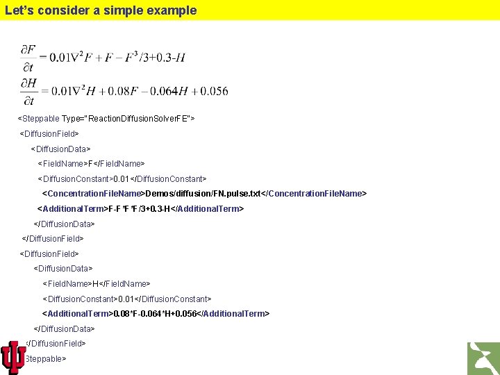
Reaction-Diffusion set of PDE’s Solving general set of above PDE’s can be tricky because functions ‘f’ can have arbitrary form. There are two ways to deal with this problem: 1. For each set of PDE’s write new PDE solver. This is not a bad idea if you can do it “on the fly”. If you can write a code that automatically generates and compiles PDE solver you will see no performance degradation 2. Use fast math expression parser that will interpret mathematical expressions during run time Compu. Cell 3 D 3. 4. 1 uses the second solution. The reason was that it was the simplest to implement and also one does not have to bother about compilers installed on users machines. However such PDE solver will not be as fast as the compiled one

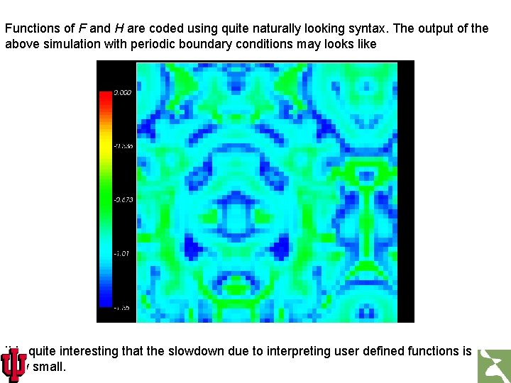
Let’s consider a simple example <Steppable Type="Reaction. Diffusion. Solver. FE"> <Diffusion. Field> <Diffusion. Data> <Field. Name>F</Field. Name> <Diffusion. Constant>0. 01</Diffusion. Constant> <Concentration. File. Name>Demos/diffusion/FN. pulse. txt</Concentration. File. Name> <Additional. Term>F-F*F*F/3+0. 3 -H</Additional. Term> </Diffusion. Data> </Diffusion. Field> <Diffusion. Data> <Field. Name>H</Field. Name> <Diffusion. Constant>0. 01</Diffusion. Constant> <Additional. Term>0. 08*F-0. 064*H+0. 056</Additional. Term> </Diffusion. Data> </Diffusion. Field> </Steppable>

Functions of F and H are coded using quite naturally looking syntax. The output of the above simulation with periodic boundary conditions may looks like It is quite interesting that the slowdown due to interpreting user defined functions is very small.

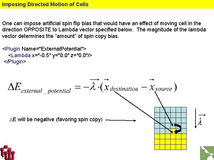
Imposing Directed Motion of Cells One can impose artificial spin flip bias that would have an effect of moving cell in the direction OPPOSITE to Lambda vector specified below. The magnitude of the lambda vector determines the “amount” of spin copy bias. <Plugin Name="External. Potential"> <Lambda x="-0. 5" y="0. 0" z="0. 0"/> </Plugin> DE will be negative (favoring spin copy)

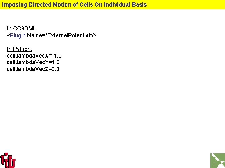
Imposing Directed Motion of Cells On Individual Basis In CC 3 DML: <Plugin Name="External. Potential“/> In Python: cell. lambda. Vec. X=-1. 0 cell. lambda. Vec. Y=1. 0 cell. lambda. Vec. Z=0. 0

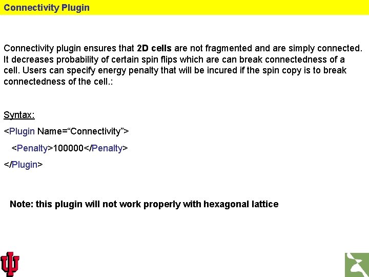
Connectivity Plugin Connectivity plugin ensures that 2 D cells are not fragmented and are simply connected. It decreases probability of certain spin flips which are can break connectedness of a cell. Users can specify energy penalty that will be incured if the spin copy is to break connectedness of the cell. : Syntax: <Plugin Name=“Connectivity”> <Penalty>100000</Penalty> </Plugin> Note: this plugin will not work properly with hexagonal lattice

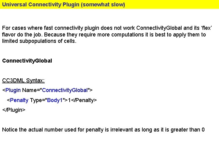
Universal Connectivity Plugin (somewhat slow) For cases where fast connectivity plugin does not work Connectivity. Global and its ‘flex’ flavor do the job. Because they require more computations it is best to apply them to limited subpopulations of cells. Connectivity. Global CC 3 DML Syntax: <Plugin Name="Connectivity. Global"> <Penalty Type="Body 1">1</Penalty> </Plugin> Notice the actual number used for penalty is irrelevant as long as it is greater than 0

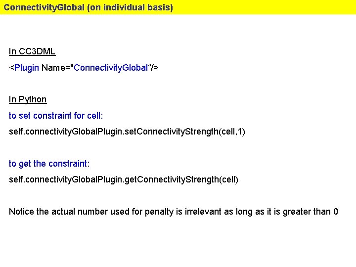
Connectivity. Global (on individual basis) In CC 3 DML <Plugin Name="Connectivity. Global“/> In Python to set constraint for cell: self. connectivity. Global. Plugin. set. Connectivity. Strength(cell, 1) to get the constraint: self. connectivity. Global. Plugin. get. Connectivity. Strength(cell) Notice the actual number used for penalty is irrelevant as long as it is greater than 0

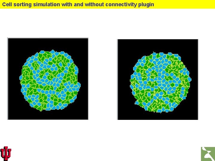
Cell sorting simulation with and without connectivity plugin

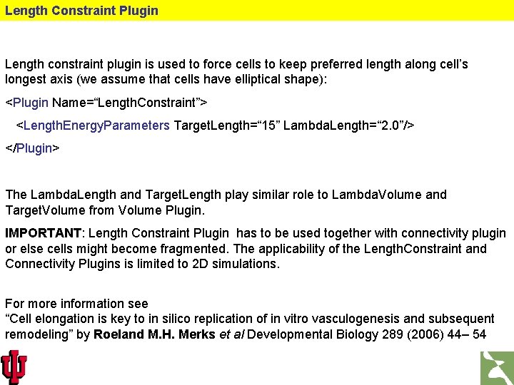
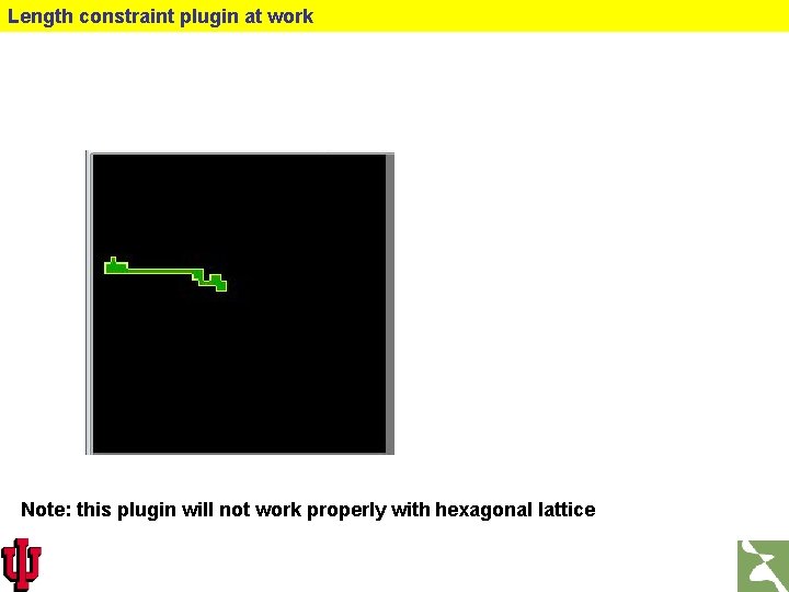
Length Constraint Plugin Length constraint plugin is used to force cells to keep preferred length along cell’s longest axis (we assume that cells have elliptical shape): <Plugin Name=“Length. Constraint”> <Length. Energy. Parameters Target. Length=“ 15” Lambda. Length=“ 2. 0”/> </Plugin> The Lambda. Length and Target. Length play similar role to Lambda. Volume and Target. Volume from Volume Plugin. IMPORTANT: Length Constraint Plugin has to be used together with connectivity plugin or else cells might become fragmented. The applicability of the Length. Constraint and Connectivity Plugins is limited to 2 D simulations. For more information see “Cell elongation is key to in silico replication of in vitro vasculogenesis and subsequent remodeling” by Roeland M. H. Merks et al Developmental Biology 289 (2006) 44– 54

Length constraint plugin at work Note: this plugin will not work properly with hexagonal lattice