INTEREST RATE DERIVATIVES THE STANDARD MARKET MODELS Chapter

INTEREST RATE DERIVATIVES: THE STANDARD MARKET MODELS Chapter 28 1

THE COMPLICATIONS IN VALUING INTEREST RATE DERIVATIVES (PAGE 647) We need a whole term structure to define the level of interest rates at any time The stochastic process for an interest rate is more complicated than that for a stock price Volatilities of different points on the term structure are different Interest rates are used for discounting the payoff as well as for defining the payoff 2

APPROACHES TO PRICING INTEREST RATE OPTIONS Use a variant of Black’s model Use a no-arbitrage (yield curve based) model 3

BLACK’S MODEL Similar to the model proposed by Fischer Black for valuing options on futures Assumes that the value of an interest rate, a bond price, or some other variable at a particular time T in the future has a lognormal distribution 4

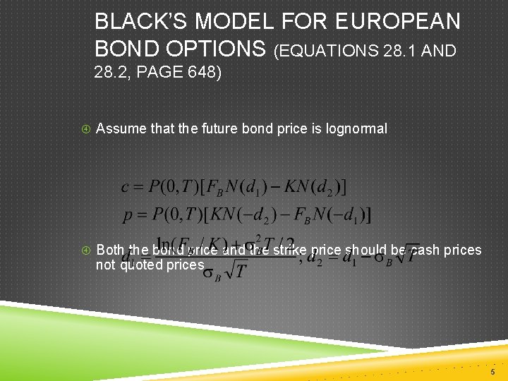
BLACK’S MODEL FOR EUROPEAN BOND OPTIONS (EQUATIONS 28. 1 AND 28. 2, PAGE 648) Assume that the future bond price is lognormal Both the bond price and the strike price should be cash prices not quoted prices 5

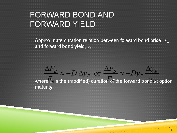
FORWARD BOND AND FORWARD YIELD Approximate duration relation between forward bond price, FB, and forward bond yield, y. F where D is the (modified) duration of the forward bond at option maturity 6

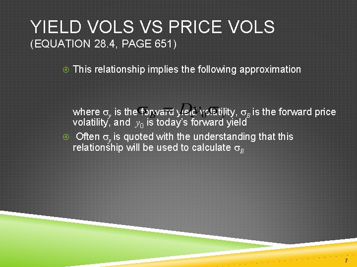
YIELD VOLS VS PRICE VOLS (EQUATION 28. 4, PAGE 651) This relationship implies the following approximation where sy is the forward yield volatility, s. B is the forward price volatility, and y 0 is today’s forward yield Often sy is quoted with the understanding that this relationship will be used to calculate s. B 7

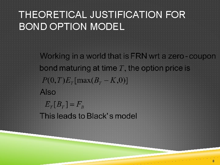
THEORETICAL JUSTIFICATION FOR BOND OPTION MODEL 8

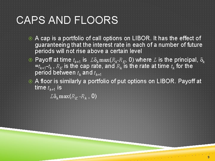
CAPS AND FLOORS A cap is a portfolio of call options on LIBOR. It has the effect of guaranteeing that the interest rate in each of a number of future periods will not rise above a certain level Payoff at time tk+1 is Ldk max(Rk-RK, 0) where L is the principal, dk =tk+1 -tk , RK is the cap rate, and Rk is the rate at time tk for the period between tk and tk+1 A floor is similarly a portfolio of put options on LIBOR. Payoff at time tk+1 is Ldk max(RK -Rk , 0) 9

CAPLETS A cap is a portfolio of “caplets” Each caplet is a call option on a future LIBOR rate with the payoff occurring in arrears When using Black’s model we assume that the interest rate underlying each caplet is lognormal 10

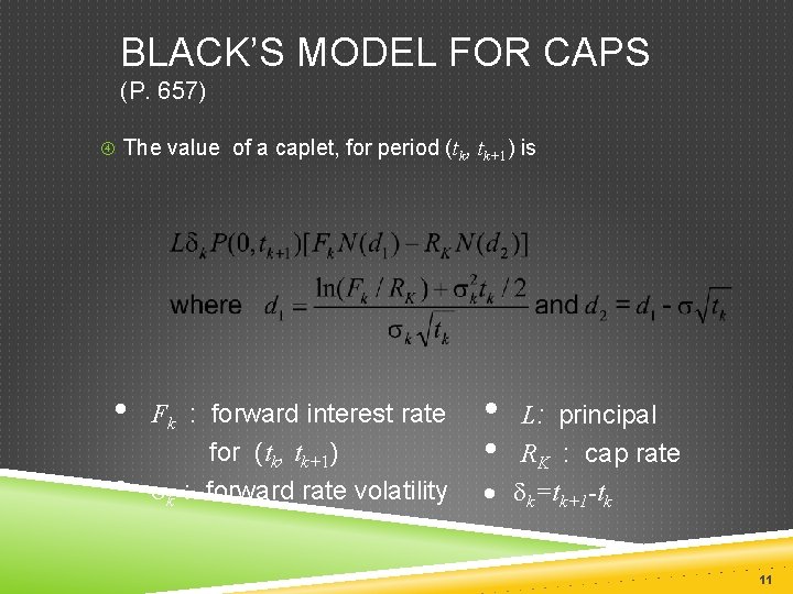
BLACK’S MODEL FOR CAPS (P. 657) The value of a caplet, for period (tk, tk+1) is • • Fk : forward interest rate for (tk, tk+1) sk : forward rate volatility • L: principal • RK : cap rate · dk=tk+1 -tk 11

WHEN APPLYING BLACK’S MODEL TO CAPS WE MUST. . . EITHER Use spot volatilities Volatility different for each caplet OR Use flat volatilities Volatility same for each caplet within a particular cap but varies according to life of cap 12

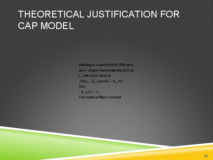
THEORETICAL JUSTIFICATION FOR CAP MODEL 13

SWAPTIONS A swaption or swap option gives the holder the right to enter into an interest rate swap in the future Two kinds The right to pay a specified fixed rate and receive LIBOR The right to receive a specified fixed rate and pay LIBOR 14

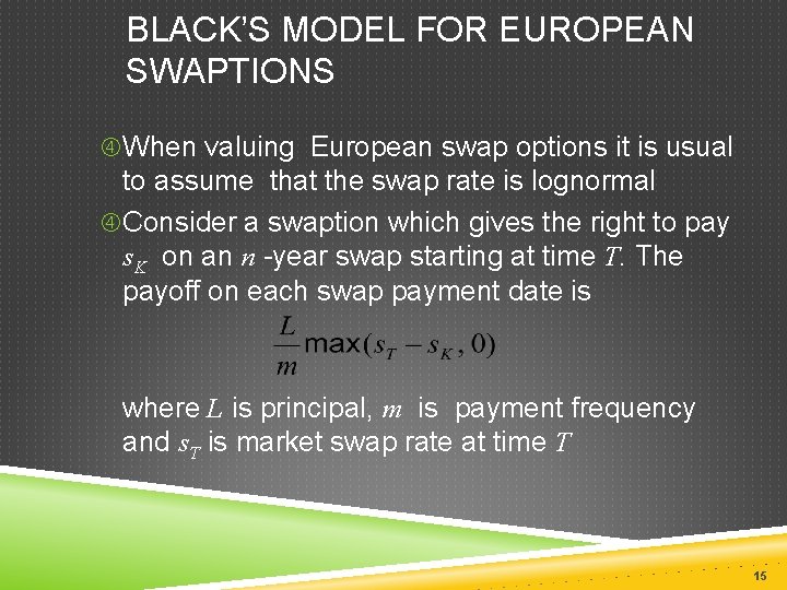
BLACK’S MODEL FOR EUROPEAN SWAPTIONS When valuing European swap options it is usual to assume that the swap rate is lognormal Consider a swaption which gives the right to pay s. K on an n -year swap starting at time T. The payoff on each swap payment date is where L is principal, m is payment frequency and s. T is market swap rate at time T 15

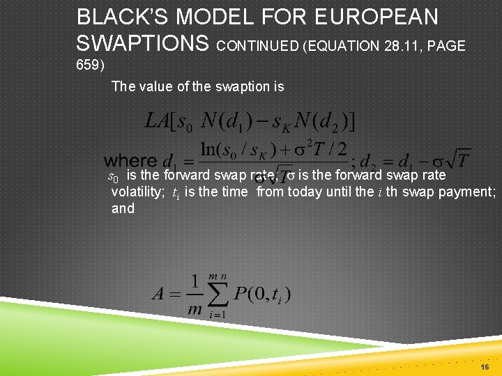
BLACK’S MODEL FOR EUROPEAN SWAPTIONS CONTINUED (EQUATION 28. 11, PAGE 659) The value of the swaption is s 0 is the forward swap rate; s is the forward swap rate volatility; ti is the time from today until the i th swap payment; and 16

THEORETICAL JUSTIFICATION FOR SWAP OPTION MODEL 17

RELATIONSHIP BETWEEN SWAPTIONS AND BOND OPTIONS An interest rate swap can be regarded as the exchange of a fixed-rate bond for a floating-rate bond A swaption or swap option is therefore an option to exchange a fixed-rate bond for a floating-rate bond 18

RELATIONSHIP BETWEEN SWAPTIONS AND BOND OPTIONS (CONTINUED) At the start of the swap the floating-rate bond is worth par so that the swaption can be viewed as an option to exchange a fixed-rate bond for par An option on a swap where fixed is paid and floating is received is a put option on the bond with a strike price of par When floating is paid and fixed is received, it is a call option on the bond with a strike price of par 19

DELTAS OF INTEREST RATE DERIVATIVES Alternatives: Calculate a DV 01 (the impact of a 1 bps parallel shift in the zero curve) Calculate impact of small change in the quote for each instrument used to calculate the zero curve Divide zero curve (or forward curve) into buckets and calculate the impact of a shift in each bucket Carry out a principal components analysis for changes in the zero curve. Calculate delta with respect to each of the first two or three factors 20

QUANTO, TIMING, AND CONVEXITY ADJUSTMENTS Chapter 29 21

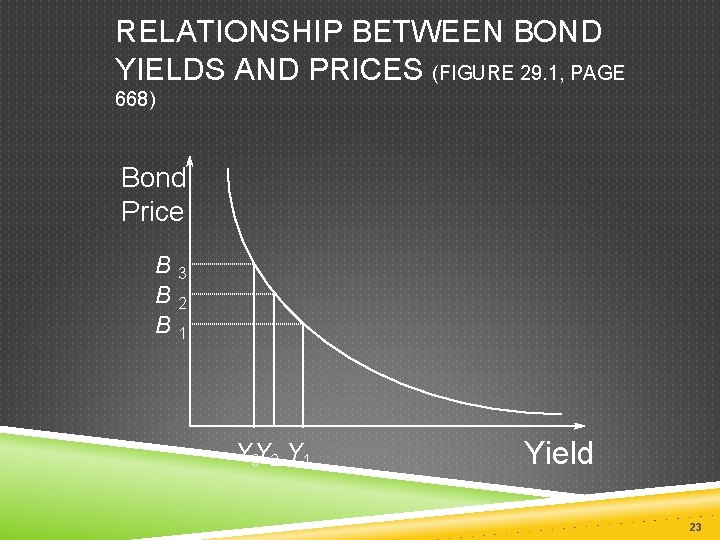
FORWARD YIELDS AND FORWARD PRICES We define the forward yield on a bond as the yield calculated from the forward bond price There is a non-linear relation between bond yields and bond prices It follows that when the forward bond price equals the expected future bond price, the forward yield does not necessarily equal the expected future yield 22

RELATIONSHIP BETWEEN BOND YIELDS AND PRICES (FIGURE 29. 1, PAGE 668) Bond Price B 3 B 2 B 1 Y 3 Y 2 Y 1 Yield 23

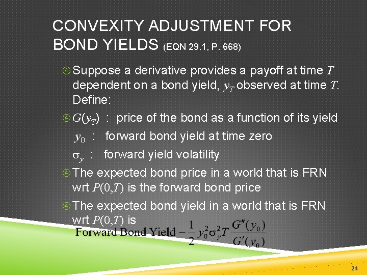
CONVEXITY ADJUSTMENT FOR BOND YIELDS (EQN 29. 1, P. 668) Suppose a derivative provides a payoff at time T dependent on a bond yield, y. T observed at time T. Define: G(y. T) : price of the bond as a function of its yield y 0 : forward bond yield at time zero sy : forward yield volatility The expected bond price in a world that is FRN wrt P(0, T) is the forward bond price The expected bond yield in a world that is FRN wrt P(0, T) is 24

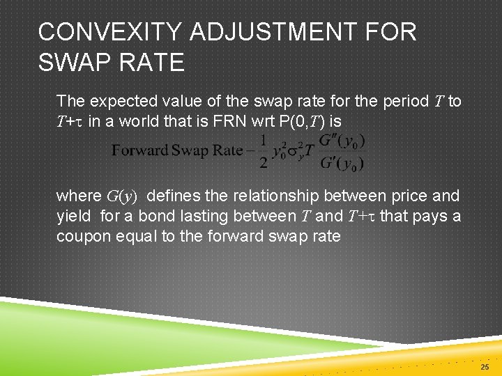
CONVEXITY ADJUSTMENT FOR SWAP RATE The expected value of the swap rate for the period T to T+t in a world that is FRN wrt P(0, T) is where G(y) defines the relationship between price and yield for a bond lasting between T and T+t that pays a coupon equal to the forward swap rate 25

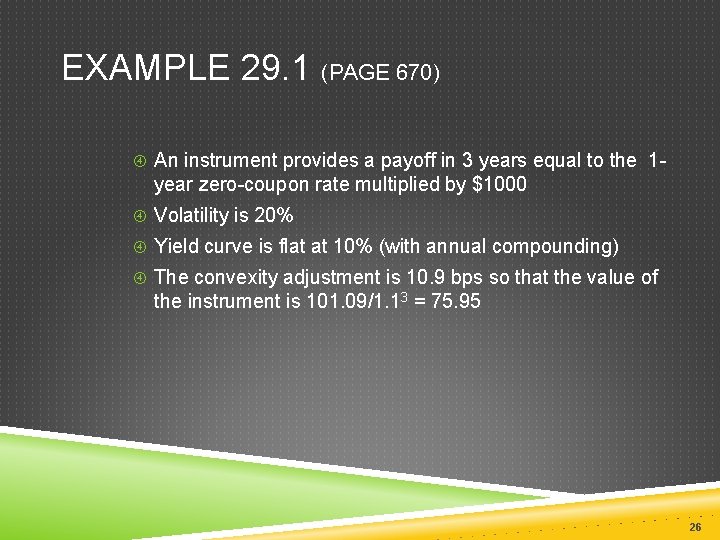
EXAMPLE 29. 1 (PAGE 670) An instrument provides a payoff in 3 years equal to the 1 - year zero-coupon rate multiplied by $1000 Volatility is 20% Yield curve is flat at 10% (with annual compounding) The convexity adjustment is 10. 9 bps so that the value of the instrument is 101. 09/1. 13 = 75. 95 26

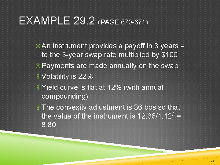
EXAMPLE 29. 2 (PAGE 670 -671) An instrument provides a payoff in 3 years = to the 3 -year swap rate multiplied by $100 Payments are made annually on the swap Volatility is 22% Yield curve is flat at 12% (with annual compounding) The convexity adjustment is 36 bps so that the value of the instrument is 12. 36/1. 123 = 8. 80 27

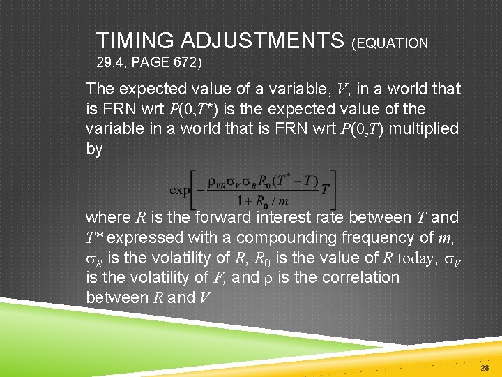
TIMING ADJUSTMENTS (EQUATION 29. 4, PAGE 672) The expected value of a variable, V, in a world that is FRN wrt P(0, T*) is the expected value of the variable in a world that is FRN wrt P(0, T) multiplied by where R is the forward interest rate between T and T* expressed with a compounding frequency of m, s. R is the volatility of R, R 0 is the value of R today, s. V is the volatility of F, and r is the correlation between R and V 28

EXAMPLE 29. 3 (PAGE 672) A derivative provides a payoff 6 years equal to the value of a stock index in 5 years. The interest rate is 8% with annual compounding 1200 is the 5 -year forward value of the stock index This is the expected value in a world that is FRN wrt P(0, 5) To get the value in a world that is FRN wrt P(0, 6) we multiply by 1. 00535 The value of the derivative is 1200× 1. 00535/(1. 086) or 760. 26 29

QUANTOS (SECTION 29. 3, PAGE 673) Quantos are derivatives where the payoff is defined using variables measured in one currency and paid in another currency Example: contract providing a payoff of ST – K dollars ($) where S is the Nikkei stock index (a yen number) 30

DIFF SWAP Diff swaps are a type of quanto A floating rate is observed in one currency and applied to a principal in another currency 31

QUANTO ADJUSTMENT (PAGE 674) The expected value of a variable, V, in a world that is FRN wrt PX(0, T) is its expected value in a world that is FRN wrt PY(0, T) multiplied by exp(r. VWs. Vs. WT) W is the forward exchange rate (units of Y per unit of X) and r. VW is the correlation between V and W. 32

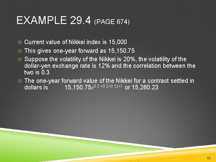
EXAMPLE 29. 4 (PAGE 674) Current value of Nikkei index is 15, 000 This gives one-year forward as 15, 150. 75 Suppose the volatility of the Nikkei is 20%, the volatility of the dollar-yen exchange rate is 12% and the correlation between the two is 0. 3 The one-year forward value of the Nikkei for a contract settled in dollars is 15, 150. 75 e 0. 3 × 0. 2× 0. 12× 1 or 15, 260. 23 33

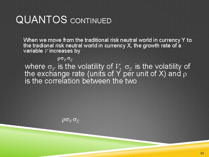
QUANTOS CONTINUED When we move from the traditional risk neutral world in currency Y to the tradional risk neutral world in currency X, the growth rate of a variable V increases by rs. V s. S where s. V is the volatility of V, s. S is the volatility of the exchange rate (units of Y per unit of X) and r is the correlation between the two rs. V s. S 34

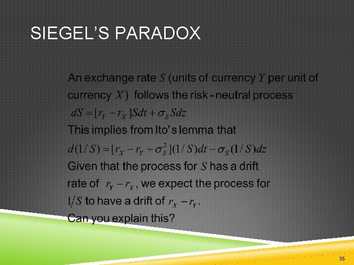
SIEGEL’S PARADOX 35

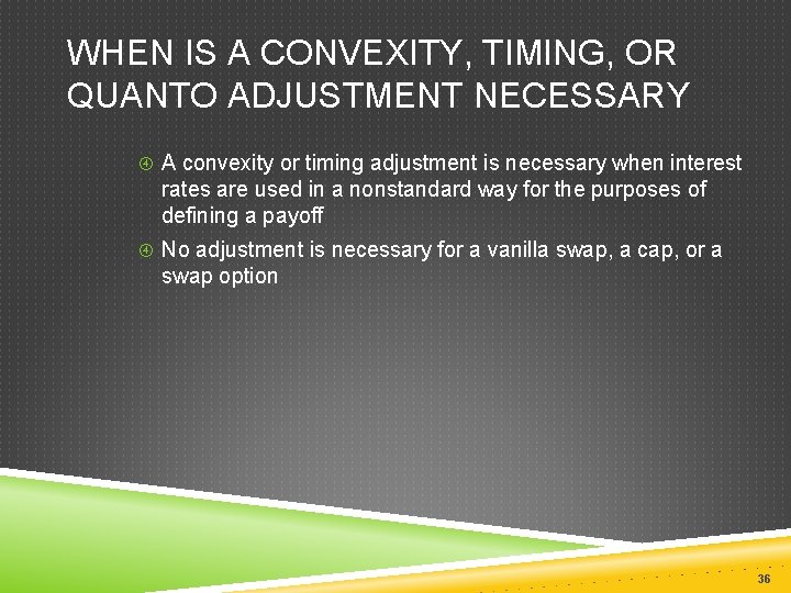
WHEN IS A CONVEXITY, TIMING, OR QUANTO ADJUSTMENT NECESSARY A convexity or timing adjustment is necessary when interest rates are used in a nonstandard way for the purposes of defining a payoff No adjustment is necessary for a vanilla swap, a cap, or a swap option 36

INTEREST RATE DERIVATIVES: MODEL OF THE SHORT RATE Chapter 30 37

TERM STRUCTURE MODELS Black’s model is concerned with describing the probability distribution of a single variable at a single point in time A term structure model describes the evolution of the whole yield curve 38

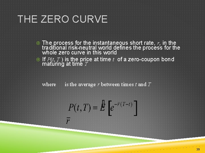
THE ZERO CURVE The process for the instantaneous short rate, r, in the traditional risk-neutral world defines the process for the whole zero curve in this world If P(t, T ) is the price at time t of a zero-coupon bond maturing at time T where is the average r between times t and T 39

EQUILIBRIUM MODELS 40

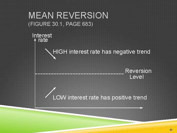
MEAN REVERSION (FIGURE 30. 1, PAGE 683) Interest rate HIGH interest rate has negative trend Reversion Level LOW interest rate has positive trend 41

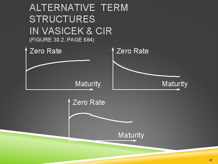
ALTERNATIVE TERM STRUCTURES IN VASICEK & CIR (FIGURE 30. 2, PAGE 684) Zero Rate Maturity 42

EQUILIBRIUM VS NO-ARBITRAGE MODELS In an equilibrium model today’s term structure is an output In a no-arbitrage model today’s term structure is an input 43

DEVELOPING NO-ARBITRAGE MODEL FOR R A model for r can be made to fit the initial term structure by including a function of time in the drift 44

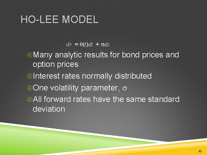
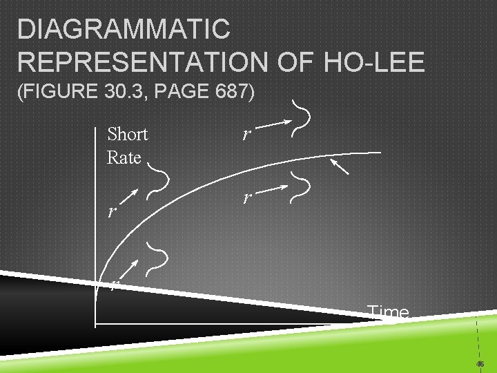
HO-LEE MODEL dr = q(t)dt + sdz Many analytic results for bond prices and option prices Interest rates normally distributed One volatility parameter, s All forward rates have the same standard deviation 45

DIAGRAMMATIC REPRESENTATION OF HO-LEE (FIGURE 30. 3, PAGE 687) Short Rate r r Time 46

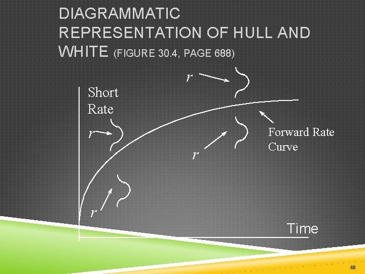
HULL-WHITE MODEL dr = [q(t ) – ar ]dt + sdz Many analytic results for bond prices and option prices Two volatility parameters, a and s Interest rates normally distributed Standard deviation of a forward rate is a declining function of its maturity 47

DIAGRAMMATIC REPRESENTATION OF HULL AND WHITE (FIGURE 30. 4, PAGE 688) Short Rate r r Forward Rate Curve Time 48

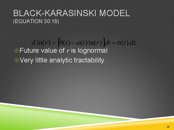
BLACK-KARASINSKI MODEL (EQUATION 30. 18) Future value of r is lognormal Very little analytic tractability 49

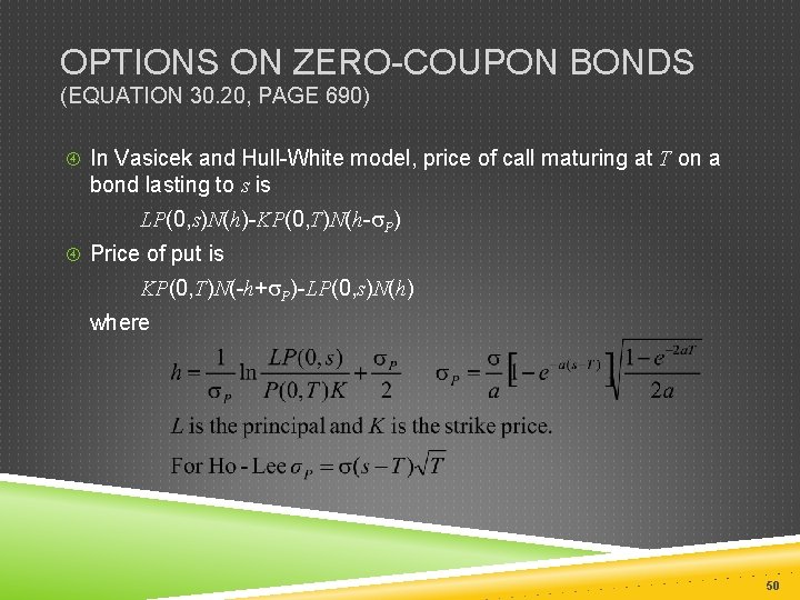
OPTIONS ON ZERO-COUPON BONDS (EQUATION 30. 20, PAGE 690) In Vasicek and Hull-White model, price of call maturing at T on a bond lasting to s is LP(0, s)N(h)-KP(0, T)N(h-s. P) Price of put is KP(0, T)N(-h+s. P)-LP(0, s)N(h) where 50

OPTIONS ON COUPON BEARING BONDS �In a one-factor model a European option on a coupon-bearing bond can be expressed as a portfolio of options on zero-coupon bonds. �We first calculate the critical interest rate at the option maturity for which the coupon-bearing bond price equals the strike price at maturity �The strike price for each zero-coupon bond is set equal to its value when the interest rate equals this critical value 51

INTEREST RATE TREES VS STOCK PRICE TREES The variable at each node in an interest rate tree is the Dt-period rate Interest rate trees work similarly to stock price trees except that the discount rate used varies from node to node 52

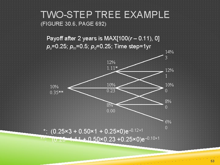
TWO-STEP TREE EXAMPLE (FIGURE 30. 6, PAGE 692) Payoff after 2 years is MAX[100(r – 0. 11), 0] pu=0. 25; pm=0. 5; pd=0. 25; Time step=1 yr 12% 1. 11* 10% 0. 35** 10% 0. 23 8% 0. 00 *: (0. 25× 3 + 0. 50× 1 + 0. 25× 0)e– 0. 12× 1 **: (0. 25× 1. 11 + 0. 50× 0. 23 +0. 25× 0)e– 0. 10× 1 14% 3 12% 1 10% 0 8% 0 6% 0 53

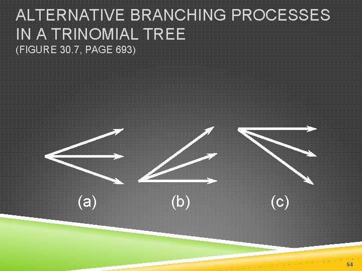
ALTERNATIVE BRANCHING PROCESSES IN A TRINOMIAL TREE (FIGURE 30. 7, PAGE 693) (a) (b) (c) 54

PROCEDURE FOR BUILDING TREE dr = [q(t ) – ar ]dt + sdz 1. Assume q(t ) = 0 and r (0) = 0 2. Draw a trinomial tree for r to match the mean and standard deviation of the process for r 3. Determine q(t ) one step at a time so that the tree matches the initial term structure 55

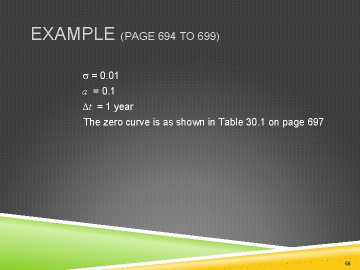
EXAMPLE (PAGE 694 TO 699) s = 0. 01 a = 0. 1 Dt = 1 year The zero curve is as shown in Table 30. 1 on page 697 56

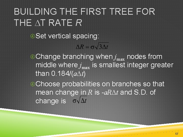
BUILDING THE FIRST TREE FOR THE DT RATE R Set vertical spacing: Change branching when jmax nodes from middle where jmax is smallest integer greater than 0. 184/(a. Dt) Choose probabilities on branches so that mean change in R is -a. RDt and S. D. of change is 57

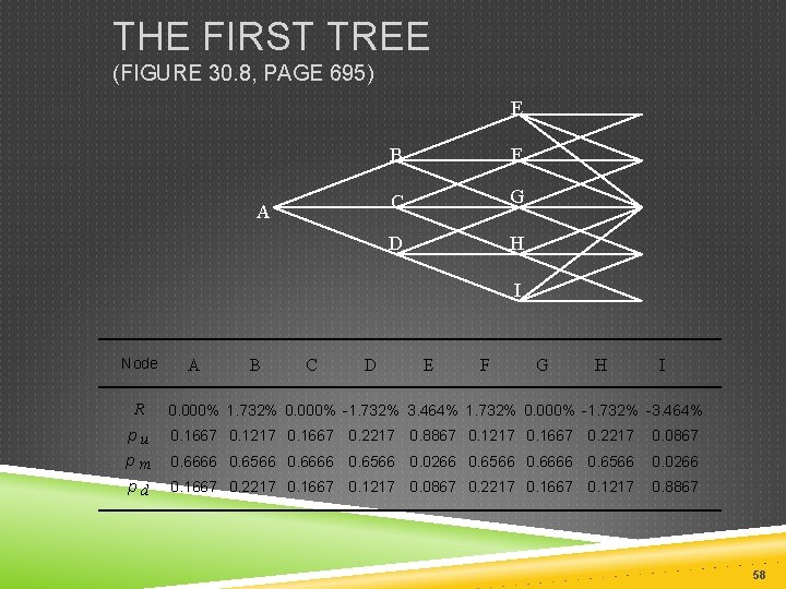
THE FIRST TREE (FIGURE 30. 8, PAGE 695) E A B F C G D H I Node R A B C D E F G H I 0. 000% 1. 732% 0. 000% -1. 732% 3. 464% 1. 732% 0. 000% -1. 732% -3. 464% pu pm 0. 1667 0. 1217 0. 1667 0. 2217 0. 8867 0. 1217 0. 1667 0. 2217 0. 0867 0. 6666 0. 6566 0. 0266 0. 6566 0. 6666 0. 6566 0. 0266 pd 0. 1667 0. 2217 0. 1667 0. 1217 0. 0867 0. 2217 0. 1667 0. 1217 0. 8867 58

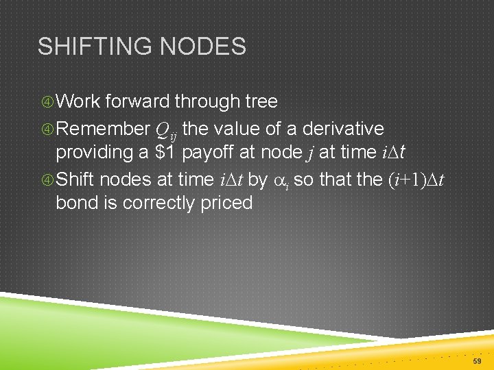
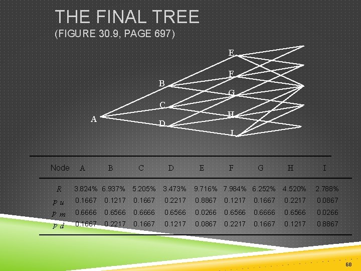
SHIFTING NODES Work forward through tree Remember Qij the value of a derivative providing a $1 payoff at node j at time i. Dt Shift nodes at time i. Dt by ai so that the (i+1)Dt bond is correctly priced 59

THE FINAL TREE (FIGURE 30. 9, PAGE 697) E F B G C A Node R pu pm pd A H D B C I D E F G H I 3. 824% 6. 937% 5. 205% 3. 473% 9. 716% 7. 984% 6. 252% 4. 520% 2. 788% 0. 1667 0. 1217 0. 1667 0. 2217 0. 8867 0. 1217 0. 1667 0. 2217 0. 0867 0. 6666 0. 6566 0. 0266 0. 6566 0. 6666 0. 6566 0. 0266 0. 1667 0. 2217 0. 1667 0. 1217 0. 0867 0. 2217 0. 1667 0. 1217 0. 8867 60

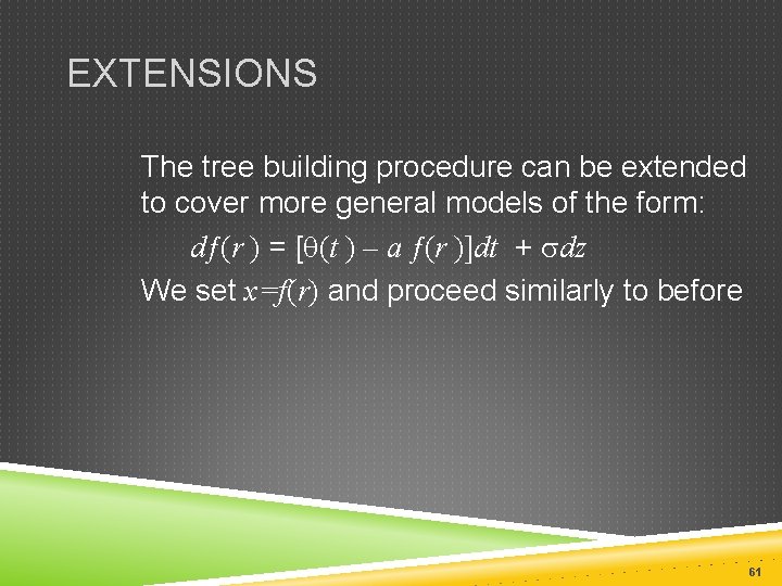
EXTENSIONS The tree building procedure can be extended to cover more general models of the form: dƒ(r ) = [q(t ) – a ƒ(r )]dt + sdz We set x=f(r) and proceed similarly to before 61

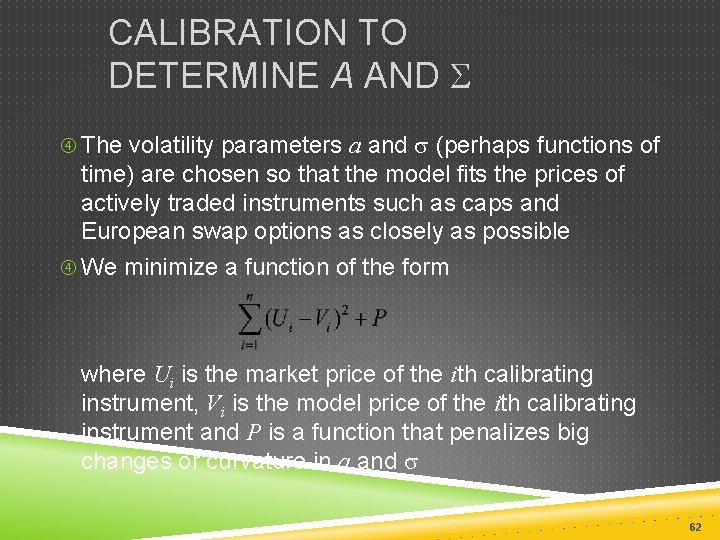
CALIBRATION TO DETERMINE A AND S The volatility parameters a and s (perhaps functions of time) are chosen so that the model fits the prices of actively traded instruments such as caps and European swap options as closely as possible We minimize a function of the form where Ui is the market price of the ith calibrating instrument, Vi is the model price of the ith calibrating instrument and P is a function that penalizes big changes or curvature in a and s 62

INTEREST RATE DERIVATIVES: HJM AND LMM Chapter 31 63

HJM MODEL: NOTATION P(t, T ): price at time t of a discount bond with principal of $1 maturing at T Wt : vector of past and present values of interest rates and bond prices at time t that are relevant for determining bond price volatilities at that time v(t, T, Wt ): volatility of P(t, T) 64

NOTATION CONTINUED ƒ(t, T 1, T 2): forward rate as seen at t for the period between T 1 and T 2 F(t, T): instantaneous forward rate as seen at t for a contract maturing at T r(t): short-term risk-free interest rate at t dz(t): Wiener process driving term structure movements 65

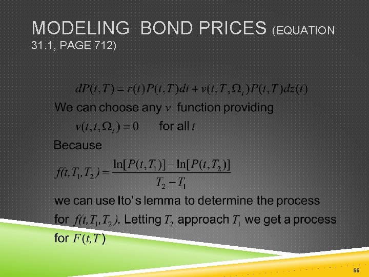
MODELING BOND PRICES (EQUATION 31. 1, PAGE 712) 66

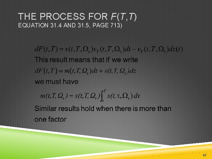
THE PROCESS FOR F(T, T) EQUATION 31. 4 AND 31. 5, PAGE 713) 67

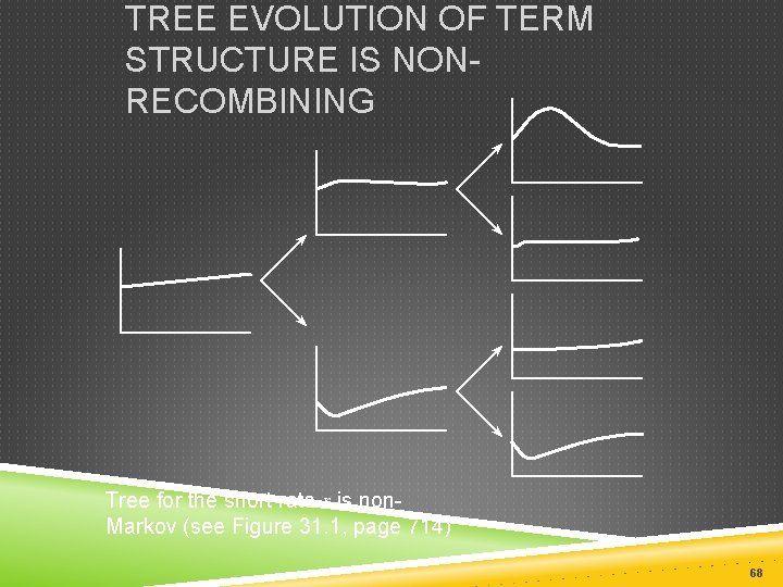
TREE EVOLUTION OF TERM STRUCTURE IS NONRECOMBINING Tree for the short rate r is non. Markov (see Figure 31. 1, page 714) 68

THE LIBOR MARKET MODEL The LIBOR market model is a model constructed in terms of the forward rates underlying caplet prices 69

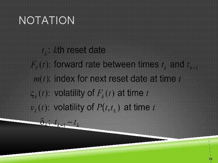
NOTATION 70

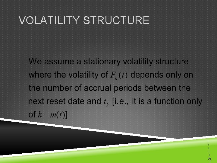
VOLATILITY STRUCTURE 71

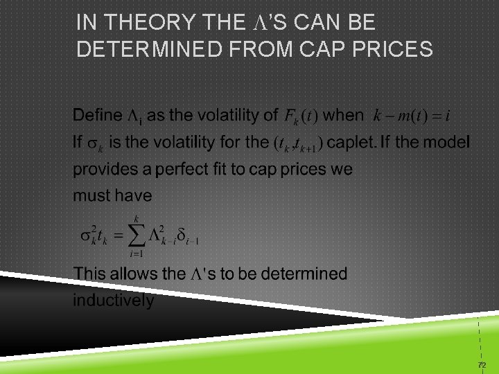
IN THEORY THE L’S CAN BE DETERMINED FROM CAP PRICES 72

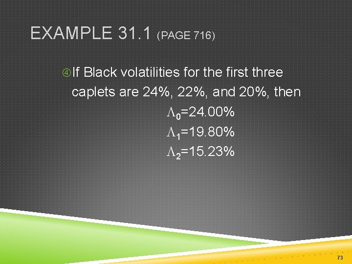
EXAMPLE 31. 1 (PAGE 716) If Black volatilities for the first three caplets are 24%, 22%, and 20%, then L 0=24. 00% L 1=19. 80% L 2=15. 23% 73

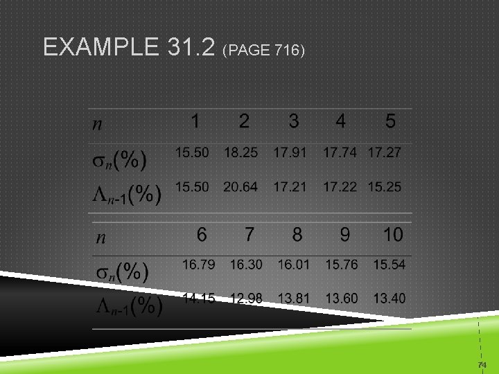
EXAMPLE 31. 2 (PAGE 716) 74

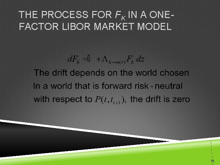
THE PROCESS FOR FK IN A ONEFACTOR LIBOR MARKET MODEL 75

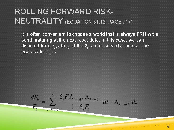
ROLLING FORWARD RISKNEUTRALITY (EQUATION 31. 12, PAGE 717) It is often convenient to choose a world that is always FRN wrt a bond maturing at the next reset date. In this case, we can discount from ti+1 to ti at the di rate observed at time ti. The process for Fk is 76

THE LIBOR MARKET MODEL AND HJM In the limit as the time between resets tends to zero, the LIBOR market model with rolling forward risk neutrality becomes the HJM model in the traditional risk-neutral world 77

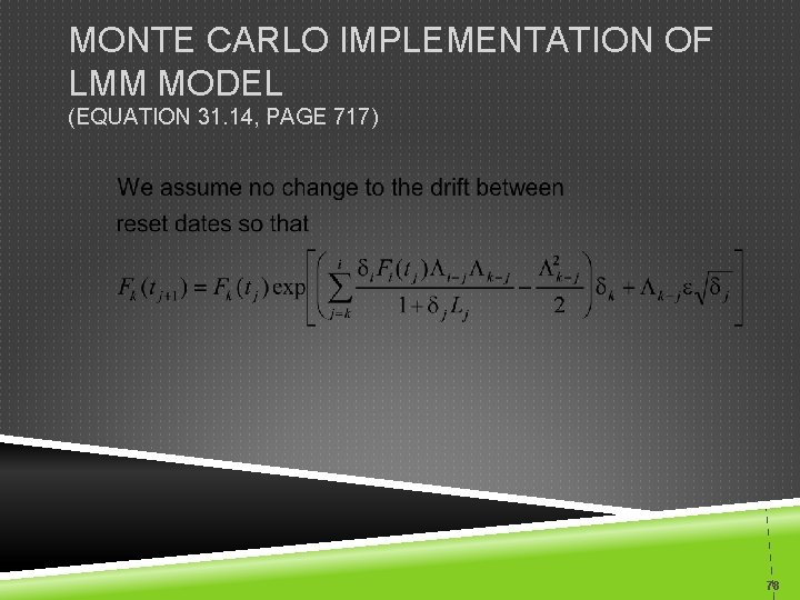
MONTE CARLO IMPLEMENTATION OF LMM MODEL (EQUATION 31. 14, PAGE 717) 78

MULTIFACTOR VERSIONS OF LMM can be extended so that there are several components to the volatility A factor analysis can be used to determine how the volatility of Fk is split into components 79

RATCHET CAPS, STICKY CAPS, AND FLEXI CAPS A plain vanilla cap depends only on one forward rate. Its price is not dependent on the number of factors. Ratchet caps, sticky caps, and flexi caps depend on the joint distribution of two or more forward rates. Their prices tend to increase with the number of factors 80

VALUING EUROPEAN OPTIONS IN THE LIBOR MARKET MODEL There is an analytic approximation that can be used to value European swap options in the LIBOR market model. See equations 31. 18 and 31. 19 on page 721 81

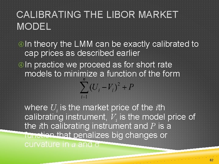
CALIBRATING THE LIBOR MARKET MODEL In theory the LMM can be exactly calibrated to cap prices as described earlier In practice we proceed as for short rate models to minimize a function of the form where Ui is the market price of the ith calibrating instrument, Vi is the model price of the ith calibrating instrument and P is a function that penalizes big changes or curvature in a and s 82

TYPES OF MORTGAGE-BACKED SECURITIES (MBSS) Pass-Through Collateralized Mortgage Obligation (CMO) Interest Only (IO) Principal Only (PO) 83

OPTION-ADJUSTED SPREAD (OAS) To calculate the OAS for an interest rate derivative we value it assuming that the initial yield curve is the Treasury curve + a spread We use an iterative procedure to calculate the spread that makes the derivative’s model price = market price. This spread is the OAS. 84