Interest Rate Derivatives Model of the Short Rate
![Hull-White Model dr = [q(t ) – ar ]dt + sdz Many analytic results Hull-White Model dr = [q(t ) – ar ]dt + sdz Many analytic results](https://slidetodoc.com/presentation_image_h2/a5cb39c6d92d63724672660850082ff3/image-11.jpg)
![Procedure for Building Tree dr = [q(t ) – ar ]dt + sdz 1. Procedure for Building Tree dr = [q(t ) – ar ]dt + sdz 1.](https://slidetodoc.com/presentation_image_h2/a5cb39c6d92d63724672660850082ff3/image-19.jpg)
- Slides: 26

Interest Rate Derivatives: Model of the Short Rate Chapter 30 Options, Futures, and Other Derivatives, 7 th Edition, Copyright © John C. Hull 2008 1

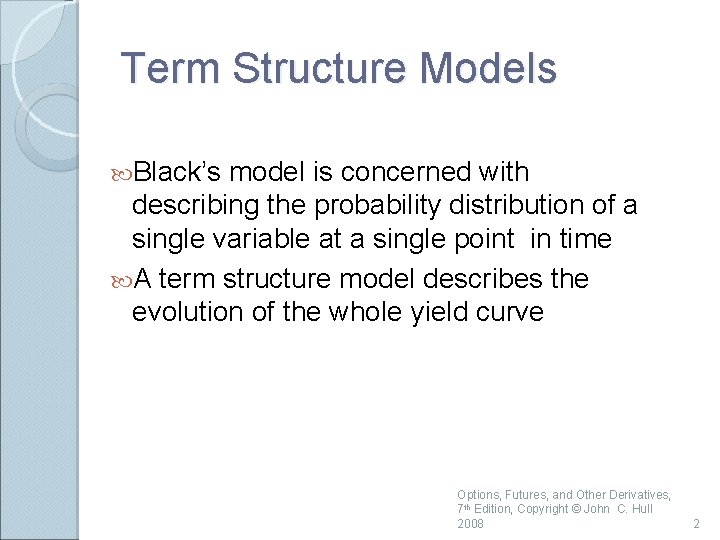
Term Structure Models Black’s model is concerned with describing the probability distribution of a single variable at a single point in time A term structure model describes the evolution of the whole yield curve Options, Futures, and Other Derivatives, 7 th Edition, Copyright © John C. Hull 2008 2

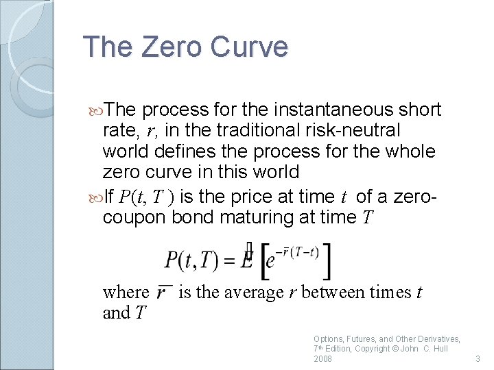
The Zero Curve The process for the instantaneous short rate, r, in the traditional risk-neutral world defines the process for the whole zero curve in this world If P(t, T ) is the price at time t of a zerocoupon bond maturing at time T where and T is the average r between times t Options, Futures, and Other Derivatives, 7 th Edition, Copyright © John C. Hull 2008 3

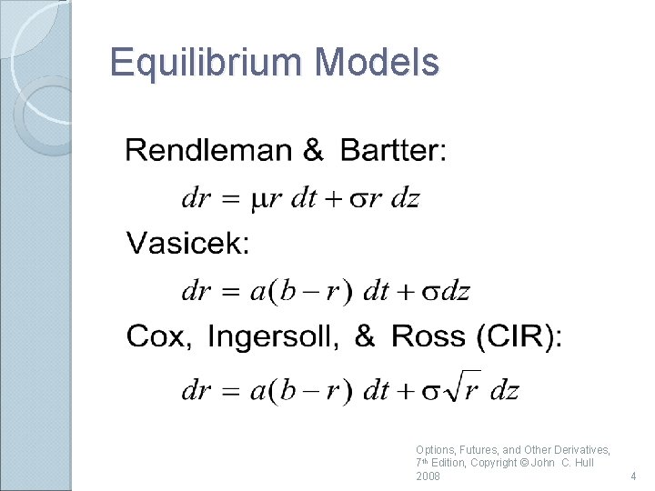
Equilibrium Models Options, Futures, and Other Derivatives, 7 th Edition, Copyright © John C. Hull 2008 4

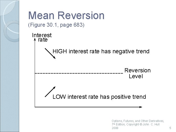
Mean Reversion (Figure 30. 1, page 683) Interest rate HIGH interest rate has negative trend Reversion Level LOW interest rate has positive trend Options, Futures, and Other Derivatives, 7 th Edition, Copyright © John C. Hull 2008 5

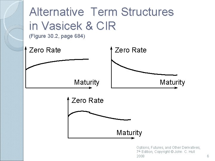
Alternative Term Structures in Vasicek & CIR (Figure 30. 2, page 684) Zero Rate Maturity Options, Futures, and Other Derivatives, 7 th Edition, Copyright © John C. Hull 2008 6

Equilibrium vs No-Arbitrage Models In an equilibrium model today’s term structure is an output In a no-arbitrage model today’s term structure is an input Options, Futures, and Other Derivatives, 7 th Edition, Copyright © John C. Hull 2008 7

Developing No-Arbitrage Model for r A model for r can be made to fit the initial term structure by including a function of time in the drift Options, Futures, and Other Derivatives, 7 th Edition, Copyright © John C. Hull 2008 8

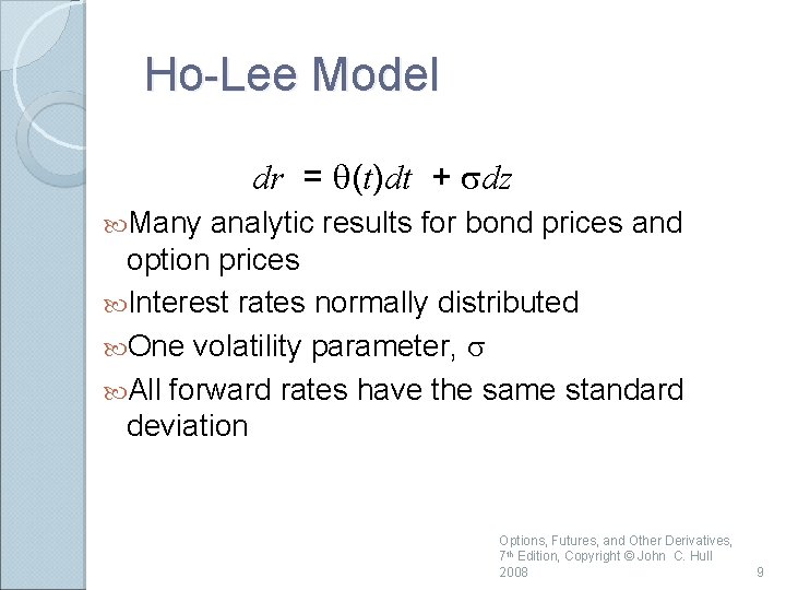
Ho-Lee Model dr = q(t)dt + sdz Many analytic results for bond prices and option prices Interest rates normally distributed One volatility parameter, s All forward rates have the same standard deviation Options, Futures, and Other Derivatives, 7 th Edition, Copyright © John C. Hull 2008 9

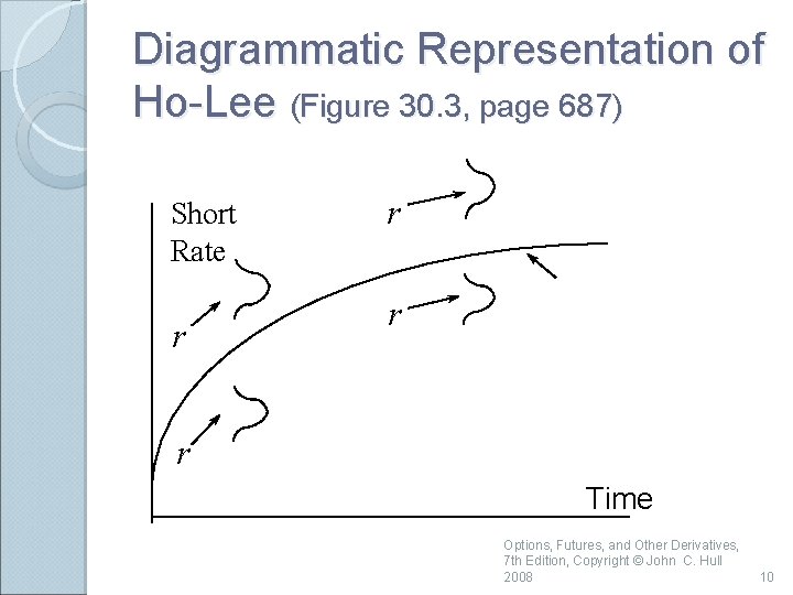
Diagrammatic Representation of Ho-Lee (Figure 30. 3, page 687) Short Rate r r Time Options, Futures, and Other Derivatives, 7 th Edition, Copyright © John C. Hull 2008 10
![HullWhite Model dr qt ar dt sdz Many analytic results Hull-White Model dr = [q(t ) – ar ]dt + sdz Many analytic results](https://slidetodoc.com/presentation_image_h2/a5cb39c6d92d63724672660850082ff3/image-11.jpg)
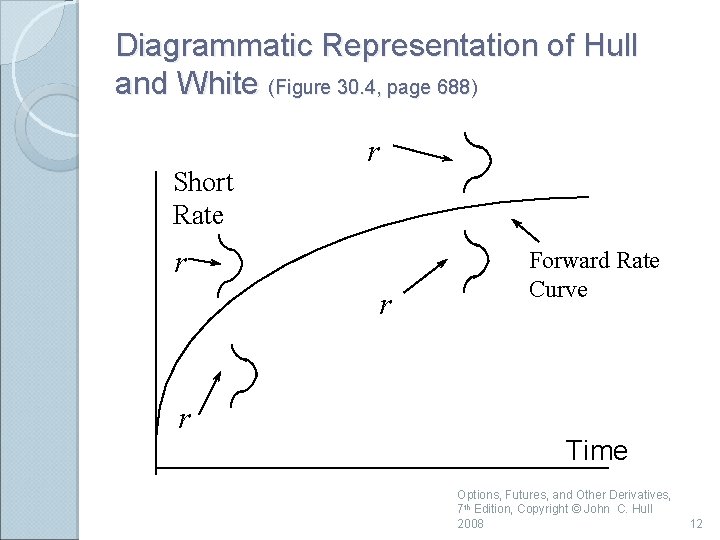
Hull-White Model dr = [q(t ) – ar ]dt + sdz Many analytic results for bond prices and option prices Two volatility parameters, a and s Interest rates normally distributed Standard deviation of a forward rate is a declining function of its maturity Options, Futures, and Other Derivatives, 7 th Edition, Copyright © John C. Hull 2008 11

Diagrammatic Representation of Hull and White (Figure 30. 4, page 688) Short Rate r r Forward Rate Curve Time Options, Futures, and Other Derivatives, 7 th Edition, Copyright © John C. Hull 2008 12

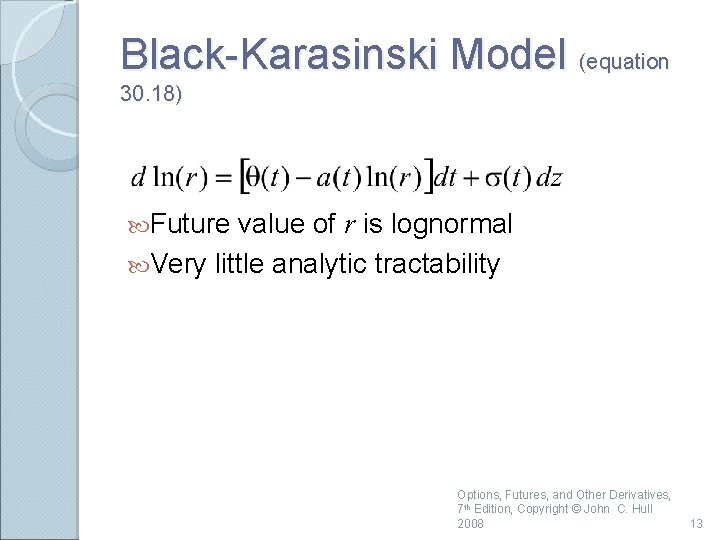
Black-Karasinski Model (equation 30. 18) Future value of r is lognormal Very little analytic tractability Options, Futures, and Other Derivatives, 7 th Edition, Copyright © John C. Hull 2008 13

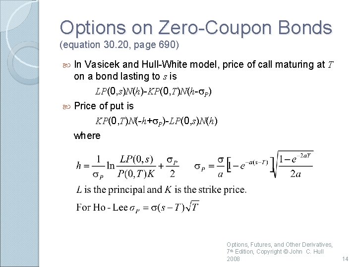
Options on Zero-Coupon Bonds (equation 30. 20, page 690) In Vasicek and Hull-White model, price of call maturing at T on a bond lasting to s is LP(0, s)N(h)-KP(0, T)N(h-s. P) Price of put is KP(0, T)N(-h+s. P)-LP(0, s)N(h) where Options, Futures, and Other Derivatives, 7 th Edition, Copyright © John C. Hull 2008 14

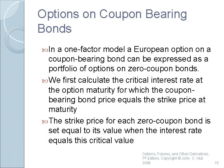
Options on Coupon Bearing Bonds In a one-factor model a European option on a coupon-bearing bond can be expressed as a portfolio of options on zero-coupon bonds. We first calculate the critical interest rate at the option maturity for which the couponbearing bond price equals the strike price at maturity The strike price for each zero-coupon bond is set equal to its value when the interest rate equals this critical value Options, Futures, and Other Derivatives, 7 th Edition, Copyright © John C. Hull 2008 15

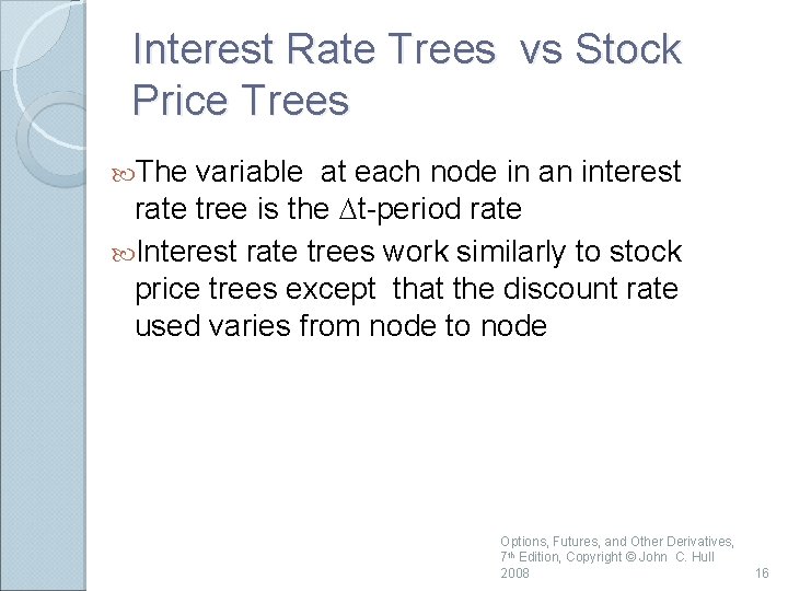
Interest Rate Trees vs Stock Price Trees The variable at each node in an interest rate tree is the Dt-period rate Interest rate trees work similarly to stock price trees except that the discount rate used varies from node to node Options, Futures, and Other Derivatives, 7 th Edition, Copyright © John C. Hull 2008 16

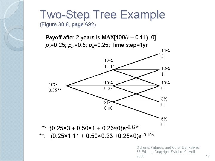
Two-Step Tree Example (Figure 30. 6, page 692) Payoff after 2 years is MAX[100(r – 0. 11), 0] pu=0. 25; pm=0. 5; pd=0. 25; Time step=1 yr 12% 1. 11* 10% 0. 35** 14% 3 12% 1 10% 0. 23 10% 0 8% 0. 00 *: (0. 25× 3 + 0. 50× 1 + 0. 25× 0)e– 0. 12× 1 **: (0. 25× 1. 11 + 0. 50× 0. 23 +0. 25× 0)e– 0. 10× 1 6% 0 Options, Futures, and Other Derivatives, 7 th Edition, Copyright © John C. Hull 2008 17

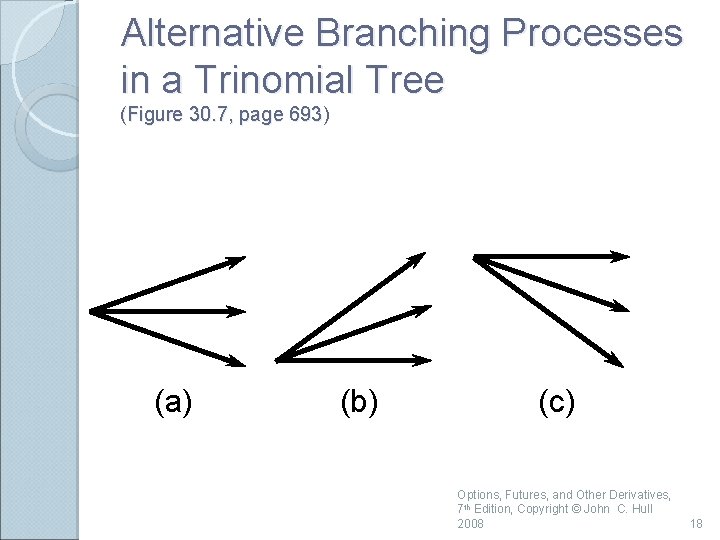
Alternative Branching Processes in a Trinomial Tree (Figure 30. 7, page 693) (a) (b) (c) Options, Futures, and Other Derivatives, 7 th Edition, Copyright © John C. Hull 2008 18
![Procedure for Building Tree dr qt ar dt sdz 1 Procedure for Building Tree dr = [q(t ) – ar ]dt + sdz 1.](https://slidetodoc.com/presentation_image_h2/a5cb39c6d92d63724672660850082ff3/image-19.jpg)
Procedure for Building Tree dr = [q(t ) – ar ]dt + sdz 1. Assume q(t ) = 0 and r (0) = 0 2. Draw a trinomial tree for r to match the mean and standard deviation of the process for r 3. Determine q(t ) one step at a time so that the tree matches the initial term structure Options, Futures, and Other Derivatives, 7 th Edition, Copyright © John C. Hull 2008 19

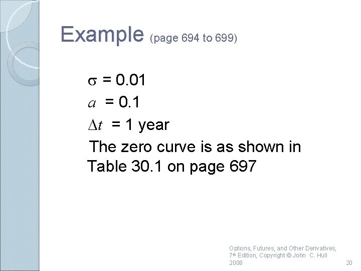
Example (page 694 to 699) s = 0. 01 a = 0. 1 Dt = 1 year The zero curve is as shown in Table 30. 1 on page 697 Options, Futures, and Other Derivatives, 7 th Edition, Copyright © John C. Hull 2008 20

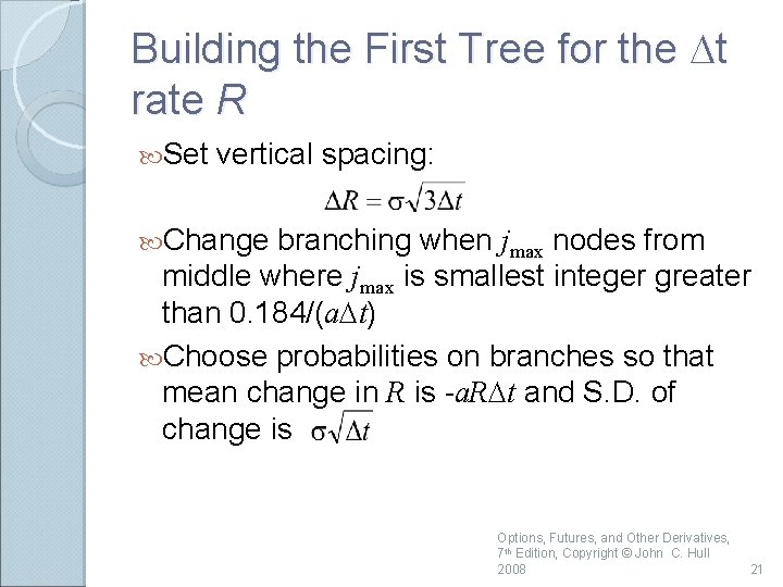
Building the First Tree for the Dt rate R Set vertical spacing: Change branching when jmax nodes from middle where jmax is smallest integer greater than 0. 184/(a. Dt) Choose probabilities on branches so that mean change in R is -a. RDt and S. D. of change is Options, Futures, and Other Derivatives, 7 th Edition, Copyright © John C. Hull 2008 21

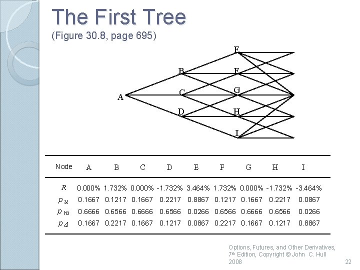
The First Tree (Figure 30. 8, page 695) E A B F C G D H I Node R A B C D E F G H I 0. 000% 1. 732% 0. 000% -1. 732% 3. 464% 1. 732% 0. 000% -1. 732% -3. 464% pu pm 0. 1667 0. 1217 0. 1667 0. 2217 0. 8867 0. 1217 0. 1667 0. 2217 0. 0867 0. 6666 0. 6566 0. 0266 0. 6566 0. 6666 0. 6566 0. 0266 pd 0. 1667 0. 2217 0. 1667 0. 1217 0. 0867 0. 2217 0. 1667 0. 1217 0. 8867 Options, Futures, and Other Derivatives, 7 th Edition, Copyright © John C. Hull 2008 22

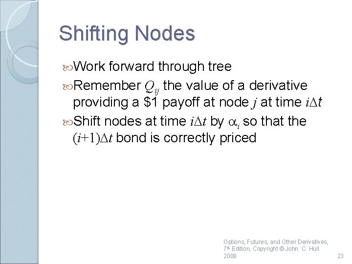
Shifting Nodes Work forward through tree Remember Qij the value of a derivative providing a $1 payoff at node j at time i. Dt Shift nodes at time i. Dt by ai so that the (i+1)Dt bond is correctly priced Options, Futures, and Other Derivatives, 7 th Edition, Copyright © John C. Hull 2008 23

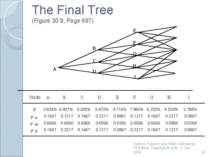
The Final Tree (Figure 30. 9, Page 697) E F B G C A Node R pu pm pd A H D B C I D E F G H I 3. 824% 6. 937% 5. 205% 3. 473% 9. 716% 7. 984% 6. 252% 4. 520% 2. 788% 0. 1667 0. 1217 0. 1667 0. 2217 0. 8867 0. 1217 0. 1667 0. 2217 0. 0867 0. 6666 0. 6566 0. 0266 0. 6566 0. 6666 0. 6566 0. 0266 0. 1667 0. 2217 0. 1667 0. 1217 0. 0867 0. 2217 0. 1667 0. 1217 0. 8867 Options, Futures, and Other Derivatives, 7 th Edition, Copyright © John C. Hull 2008 24

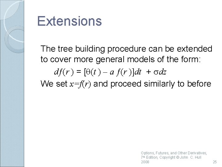
Extensions The tree building procedure can be extended to cover more general models of the form: dƒ(r ) = [q(t ) – a ƒ(r )]dt + sdz We set x=f(r) and proceed similarly to before Options, Futures, and Other Derivatives, 7 th Edition, Copyright © John C. Hull 2008 25

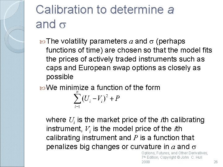
Calibration to determine a and s volatility parameters a and s (perhaps functions of time) are chosen so that the model fits the prices of actively traded instruments such as caps and European swap options as closely as possible We minimize a function of the form The where Ui is the market price of the ith calibrating instrument, Vi is the model price of the ith calibrating instrument and P is a function that penalizes big changes or curvature in a and s Options, Futures, and Other Derivatives, 7 th Edition, Copyright © John C. Hull 2008 26