Indexing The essential step in searching Review a

Indexing The essential step in searching

Review a bit • We have seen so far – Crawling • In the abstract and as implemented • Your own code and Nutch • If you are unsure about anything related to crawling, be sure to speak up now! – Collection Building • Once you have crawled, you have a collection of documents. Presumably, you want to be able to retrieve the documents that are relevant to specified information need.

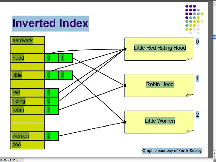
Information Retrieval • Finding the specific bit of information in the collection that satisfies a need and allows a user to complete a task. • Remember – a web search does not search the web directly. – It searches in the index created when the web pages were found analyzed. • Last class, we saw the basic structure of indexing. Review

Inverted index construction Documents to be indexed. Token stream. Modified tokens. Friends, Romans, countrymen. Tokenizer Romans Countrymen friend roman countryman Linguistic modules Stop words, stemming, capitalization, cases, etc. Inverted index. Friends Indexer friend 2 4 roman 1 2 countryman 13 16

Indexer steps: Token sequence § Sequence of (Modified token, Document ID) pairs. Initially, all the tokens from document 1, then all the tokens from document 2, etc. , without regard for duplication. Doc 1 I did enact Julius Caesar I was killed i' the Capitol; Brutus killed me. Doc 2 So let it be with Caesar. The noble Brutus hath told you Caesar was ambitious

Indexer steps: Sort § Sort by terms § doc. ID within terms Core indexing step

Indexer steps: Dictionary & Postings ID n tai on tc ha ts t en cum do the ter m Number of documents in which the term appears of § Multiple term entries in a single document are merged. § Split into Dictionary and Postings § Doc. frequency information is added.

Spot check • Complete the indexing for the following two “documents. ” – Of course, the examples have to be very small to be manageable. Imagine that you are indexing the entire news stories. – Construct the charts as seen on the previous slide – Put your solution in the Blackboard Indexing – Spot Check 1. There is a discussion board in Blackboard. You will find it on the content homepage. Document 1: Pearson and Google Jump Into Learning Management With a New, Free System Document 2: Pearson adds free learning management tools to Google Apps for Education

Problem with Boolean search: feast or famine • Boolean queries often result in either too few (=0) or too many (1000 s) results. • A query that is too broad yields hundreds of thousands of hits • A query that is too narrow may yield no hits • It takes a lot of skill to come up with a query that produces a manageable number of hits. – AND gives too few; OR gives too many

Ranked retrieval models • Rather than a set of documents satisfying a query expression, in ranked retrieval models, the system returns an ordering over the (top) documents in the collection with respect to a query • Free text queries: Rather than a query language of operators and expressions, the user’s query is just one or more words in a human language • In principle, these are different options, but in practice, ranked retrieval models have normally been associated with free text queries and vice versa 10

Feast or famine: not a problem in ranked retrieval • When a system produces a ranked result set, large result sets are not an issue – Indeed, the size of the result set is not an issue – We just show the top k ( ≈ 10) results – We don’t overwhelm the user – Premise: the ranking algorithm works

Scoring as the basis of ranked retrieval • We wish to return, in order, the documents most likely to be useful to the searcher • How can we rank-order the documents in the collection with respect to a query? • Assign a score – say in [0, 1] – to each document • This score measures how well document and query “match”.

Query-document matching scores • We need a way of assigning a score to a query/document pair • Let’s start with a one-term query • If the query term does not occur in the document: score should be 0 • The more frequent the query term in the document, the higher the score (should be) • We will look at a number of alternatives for this.

Take 1: Jaccard coefficient • A commonly used measure of overlap of two sets A and B – jaccard(A, B) = |A ∩ B| / |A ∪ B| – jaccard(A, A) = 1 – jaccard(A, B) = 0 if A ∩ B = 0 • A and B don’t have to be the same size. • Always assigns a number between 0 and 1.

Jaccard coefficient: Scoring example • What is the query-document match score that the Jaccard coefficient computes for each of the two “documents” below? • Query: ides of march • Document 1: caesar died in march • Document 2: the long march

Jaccard Example done • • • Query: ides of march Document 1: caesar died in march Document 2: the long march A = {ides, of, march} B 1 = {caesar, died, in, march} • B 2 = {the, long, march}

Issues with Jaccard for scoring • It doesn’t consider term frequency (how many times a term occurs in a document) – Rare terms in a collection are more informative than frequent terms. Jaccard doesn’t consider this information • We need a more sophisticated way of normalizing for length The problem with the first example was that document 2 “won” because it was shorter, not because it was a better match. We need a way to take into account document length so that longer documents are not penalized in calculating the match score.

Term frequency • Two factors: – A term that appears just once in a document is probably not as significant as a term that appears a number of times in the document. – A term that is common to every document in a collection is not a very good choice for choosing one document over another to address an information need. • Let’s see how we can use these two ideas to refine our indexing and our search

Term frequency - tf • The term frequency tft, d of term t in document d is defined as the number of times that t occurs in d. • We want to use tf when computing querydocument match scores. But how? • Raw term frequency is not what we want: – A document with 10 occurrences of the term is more relevant than a document with 1 occurrence of the term. – But not 10 times more relevant. • Relevance does not increase proportionally with term frequency. NB: frequency = count in IR

Log-frequency weighting • The log frequency weight of term t in d is • 0 → 0, 1 → 1, 2 → 1. 3, 10 → 2, 1000 → 4, etc. • Score for a document-query pair: sum over terms t in both q and d: score • The score is 0 if none of the query terms is present in the document.

Document frequency • Rare terms are more informative than frequent terms – Recall stop words • Consider a term in the query that is rare in the collection (e. g. , arachnocentric) • A document containing this term is very likely to be relevant to the query arachnocentric • → We want a high weight for rare terms like arachnocentric, even if the term does not appear many times in the document.

Document frequency, continued • Frequent terms are less informative than rare terms • Consider a query term that is frequent in the collection (e. g. , high, increase, line) – A document containing such a term is more likely to be relevant than a document that doesn’t – But it’s not a sure indicator of relevance. • → For frequent terms, we want high positive weights for words like high, increase, and line – But lower weights than for rare terms. • We will use document frequency (df) to capture this.

idf weight • dft is the document frequency of t: the number of documents that contain t – dft is an inverse measure of the informativeness of t – dft N (the number of documents) • We define the idf (inverse document frequency) of t by – We use log (N/dft) instead of N/dft to “dampen” the effect of idf. Will turn out the base of the log is immaterial.

idf example, suppose N = 1 million term calpurnia dft idft 1 6 animal 100 4 sunday 1, 000 3 10, 000 2 100, 000 1 1, 000 0 fly under the There is one idf value for each term t in a collection.

Effect of idf on ranking • Does idf have an effect on ranking for oneterm queries, like – i. Phone • idf has no effect on ranking one term queries – idf affects the ranking of documents for queries with at least two terms – For the query capricious person, idf weighting makes occurrences of capricious count for much more in the final document ranking than occurrences of person. 25

Collection vs. Document frequency • The collection frequency of t is the number of occurrences of t in the collection, counting multiple occurrences. • Example: Word Collection frequency Document frequency insurance 10440 3997 try 10422 8760 • Which word is a better search term (and should get a higher weight)?

tf-idf weighting • The tf-idf weight of a term is the product of its tf weight and its idf weight. • Best known weighting scheme in information retrieval – Note: the “-” in tf-idf is a hyphen, not a minus sign! – Alternative names: tf. idf, tf x idf • Increases with the number of occurrences within a document • Increases with the rarity of the term in the collection

Final ranking of documents for a query 28

Binary → count → weight matrix Each document is now represented by a real-valued vector of tf-idf weights ∈ R|V|

|V| is theas number Documents vectors of terms • So we have a |V|-dimensional vector space • Terms are axes of the space • Documents are points or vectors in this space • Very high-dimensional: tens of millions of dimensions when you apply this to a web search engine • These are very sparse vectors - most entries are zero.

Queries as vectors • Key idea 1: Do the same for queries: represent them as vectors in the space • Key idea 2: Rank documents according to their proximity to the query in this space • proximity = similarity of vectors • proximity ≈ inverse of distance • Recall: We do this because we want to get away from the you’re-either-in-or-out Boolean model. • Instead: rank more relevant documents higher than less relevant documents

Making it clear • We now see a document as a vector: a sequence of real numbers, each associated with a term that may or may not be in the document. • Every indexed term in the document collection is represented in the vector. Usually, that means a lot of vector entries.

Exercise • Open the file Search-jaguar. txt • Skip the first line, which is just a description of the page. • Treat each other entry on the page (1 to 3 lines each) as a document. – Create the dictionary (complete list of terms for all the collection. Do not eliminate any stop words, etc. ) Do merge singular and plural forms. – For each document, create its vector. • First, just do 1 or 0 – word is in the document or not. • Then compute the tf-idf weights. – It is ok to divide this up – each student create the tf-idf vector for a different document.

What is a vector? • Suppose we have only two terms in our dictionary. Suppose jaguar and car. • Suppose that two documents have the following tf-idf weights of those two terms: – Doc 1: jaguar 0. 800 – Doc 2: jaguar 0. 300 car 0. 600 car 0. 500 • How similar are those documents?

Vector space • Each document is represented by the sequence of numbers that show its weight in this two dimensional space: – Doc 1 = (0. 8, 0. 6) – Doc 2 = (0. 3, 0. 5) car We will see later how to normalize so that all weights are between 0 and 1 . 6. 5 Doc 2 Doc 1 . 3 . 8 jaguar With this representation, we can visualize (for 2 dimensions) how similar two documents are. More importantly, we can measure their similarity and compare it to the similarity of another document to one of these.

Dimensionality • We are showing only two dimensions – appropriate if there are only two terms. • There are thousands of terms, perhaps millions, in the general case. • We can apply the same measurement techniques, but we cannot draw them. • So, how shall we measure the distance between two vectors?

Formalizing vector space proximity • First cut: distance between two points ( = distance between the end points of the two vectors) • Euclidean distance? • Euclidean distance is a bad idea. . . • . . . because Euclidean distance is large for vectors of different lengths.

Why distance is a bad idea The Euclidean distance between q and d 2 is large even though the distribution of terms in the query q and the distribution of terms in the document d 2 are very similar. Note that if d 2 had fewer references to each of the terms, such that the vector length was similar to the others, it would be clearly the closest to q. Is this the result that we want?

Use angle instead of distance • Thought experiment: take a document d and append it to itself. Call this document d′ • “Semantically” d and d′ have the same content • The Euclidean distance between the two documents can be quite large • The angle between the two documents is 0, corresponding to maximal similarity. • Key idea: Rank documents according to angle with query.

From angles to cosines • The following two notions are equivalent. – Rank documents in decreasing order of the angle between query and document – Rank documents in increasing order of cosine(query, document) • Cosine is a monotonically decreasing function for the interval [0 o, 180 o]

From angles to cosines • But how – and why – should we be computing cosines?

Length normalization • A vector can be (length-) normalized by dividing each of its components by its length – for this we use the L 2 norm: • Dividing a vector by its L 2 norm makes it a unit (length) vector (on surface of unit hypersphere) • Effect on the two documents d and d′ (d appended to itself) from earlier slide: they have identical vectors after length-normalization. – Long and short documents now have comparable weights

cosine(query, document) Dot product Recall: tf gives significance to terms that appear frequently; idf gives significance to terms that are unusual over all the documents Reminder? -- Unit vectors qi is the tf-idf weight of term i in the query di is the tf-idf weight of term i in the document cos(q, d) is the cosine similarity of q and d … or, equivalently, the cosine of the angle between q and d. In mathematics, the dot product is an algebraic operation that takes two equal-length sequences of numbers (usually coordinate vectors) and returns a single number obtained by multiplying corresponding entries and then summing those products. The name is derived from the centered dot " " that is often used to designate this operation; the alternative name scalar product emphasizes the scalar (rather than vector) nature of the result. At a basic level, the dot product is used to obtain the cosine of the angle between two vectors.

Cosine for length-normalized vectors • For length-normalized vectors, cosine similarity is simply the dot product (or scalar product): for q, d length-normalized. 44

Cosine similarity illustrated 45

Cosine similarity amongst 3 documents How similar are the novels Sa. S: Sense and Sensibility Pa. P: Pride and Prejudice, and WH: Wuthering Heights? term affection Sa. S Pa. P WH 115 58 20 jealous 10 7 11 gossip 2 0 6 wuthering 0 0 38 Term frequencies (counts) Note: To simplify this example, we don’t do idf weighting.

3 documents example contd. Log frequency weighting term Sa. S Pa. P After length normalization WH term Sa. S Pa. P WH affection 3. 06 2. 76 2. 30 affection 0. 789 0. 832 0. 524 jealous 2. 00 1. 85 2. 04 jealous 0. 515 0. 555 0. 465 gossip 1. 30 0 1. 78 gossip 0. 335 0 0. 405 0 0 2. 58 wuthering 0 0 0. 588 wuthering cos(Sa. S, Pa. P) ≈ 0. 789 × 0. 832 + 0. 515 × 0. 555 + 0. 335 × 0. 0 + 0. 0 × 0. 0 ≈ 0. 94 Recall: log frequency weight is cos(Sa. S, WH) ≈ 0. 79 cos(Pa. P, WH) ≈ 0. 69 Why do we have cos(Sa. S, Pa. P) > cos(SAS, WH)?

Weighting may differ in queries vs documents • Many search engines allow for different weightings for queries vs. documents • SMART Notation: denotes the combination in use in an engine, with the notation ddd. qqq, using the acronyms from this table A very standard combination is lnc. ltc Table from Wikipedia

tf-idf example: lnc. ltc Document: car insurance auto insurance Query: best car insurance Term Query tf-wt raw df idf Document wt n’lize tf-raw tf-wt Prod wt n’lize auto 0 0 5000 2. 3 0 0 1 1 1 0. 52 0 best 1 1 50000 1. 3 0. 34 0 0 0 car 1 1 10000 2. 0 0. 52 1 1 1 0. 52 0. 27 insurance 1 1 3. 0 0. 78 2 1. 3 0. 68 0. 53 1000 Doc length = Score = 0+0+0. 27+0. 53 = 0. 8

Summary – vector space ranking • Represent the query as a weighted tf-idf vector • Represent each document as a weighted tf-idf vector • Compute the cosine similarity score for the query vector and each document vector • Rank documents with respect to the query by score • Return the top K (e. g. , K = 10) to the user

The Practical Reality • No, you don’t have to write code from scratch to do the indexing and searching functions. • Just as we found Nutch to do crawling, we can find professionally developed open source products for indexing and searching. • Let’s look briefly at Lucene and Solr. – Next week – hands on laboratory for incorporating these into your projects

Lucene – A search resource • Part of the Apache suite of web-related software. • Apache Lucene is a high-performance, fullfeatured text search engine library written entirely in Java. It is a technology suitable for nearly any application that requires fulltext search, especially cross-platform. • Apache Lucene is an open source project available for free download.

Lucene Features • Scalable, High-Performance Indexing – – over 20 MB/minute on Pentium M 1. 5 GHz small RAM requirements -- only 1 MB heap incremental indexing as fast as batch indexing index size roughly 20 -30% the size of text indexed • Powerful, Accurate and Efficient Search Algorithms – ranked searching -- best results returned first – many powerful query types: phrase queries, wildcard queries, proximity queries, range queries and more – fielded searching (e. g. , title, author, contents) – date-range searching – sorting by any field – multiple-index searching with merged results – allows simultaneous update and searching

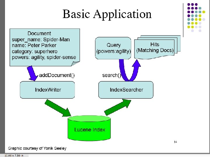
Lucene overview • Lucene provides – Indexing of your information – Search of your information, using the previously constructed index. • You provide – The user interface – The application of which the search is a part

Step by step - Index • First step - Index – Build an index of whatever you will want to search later. • Several classes (Java classes, that is) of analyzers. Choose the one that suits your need: – Standard. Analyzer » A sophisticated general-purpose analyzer. – Whitespace. Analyze » A very simple analyzer that just separates tokens using white space. – Stop. Analyzer » Removes common English words that are not usually useful for indexing. – Snowball. Analyzer » An interesting experimental analyzer that works on word roots (a search on rain should also return entries with raining, rained, and so on).

Second step - Search • After the index is built, we can search. • There are java classes provided (Index. Searcher and Query. Parser) to do just what the names suggest. • You specify the analyzer that you want to apply to the query – it must be the same analyzer that you used to build the index, not surprisingly. • You also specify the field that you want to search, and the query that the user entered, that says what you want to search for.

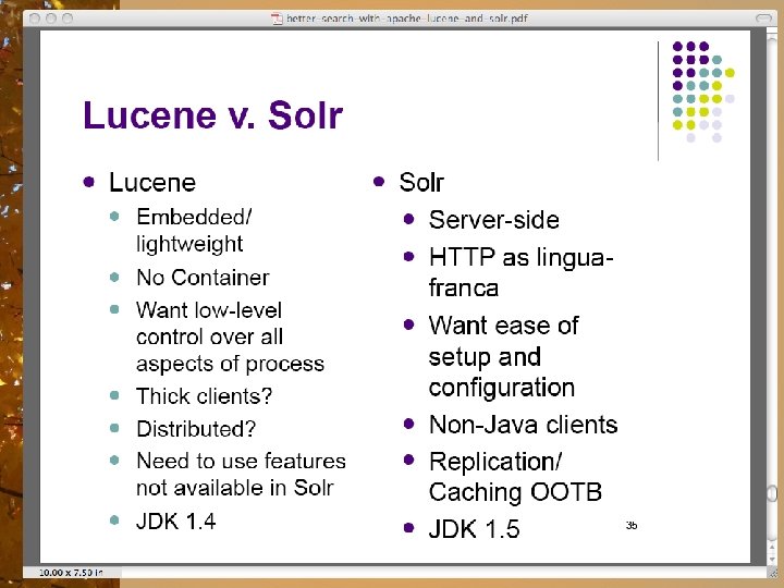
Lucene • Modified Vector Space Model of search – combines Boolean and VSM • Written in Java, but ported to many other languages • A library for enabling text-based search • Note – you must build the application – Lucene is a collection of modules to use in your application to do the indexing and searching steps

Lucene indexes strings • Not aware of markup, such as XML, HTML, Word, PDF, etc • There are good open source tools for extracting the content from marked up files – See Beautiful. Soup for HTML, for example

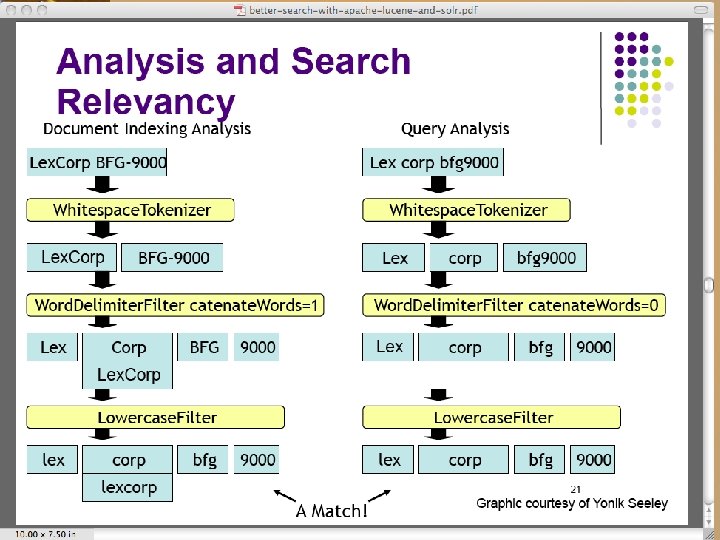
Lucene Analysis • Analysis is the process of preparing text for use in indexing and searching • Analyzer, Tokenizer, Token. Filter classes – Token. Filter can apply stemming, for example. – Several analyzers come with Lucene. Application developer chooses which to use. • Example: Whitespace. Analyzer separates tokens based on white space

Lucene - final • Lucene is a collection of java classes that implement the type of indexing and searching techniques we talk about, and that you read elsewhere. • The implementation is free, but has to be integrated into whatever application you are building to which you want to add search capability.

Solr • Built on lucene, solr is an open source search platform, also from the apache project. • Features include “powerful full-text search, hit highlighting, faceted search, dynamic clustering, database integration, and rich document (e. g. , Word, PDF) handling. Solr is highly scalable, providing distributed search and index replication, and it powers the search and navigation features of many of the world's largest internet sites. “

Resources for this material • Introduction to Information Retrieval, sections 6. 2 – 6. 4. 3 • Slides provided by the author • http: //www. miislita. com/information-retrieval -tutorial/cosine-similarity-tutorial. html -Term weighting and cosine similarity tutorial • Better Search with Apache Lucene and Solr trijug. org/downloads/Tri. Jug-11 -07. pdf