Image warpingmorphing Digital Visual Effects YungYu Chuang with

Image warping/morphing Digital Visual Effects Yung-Yu Chuang with slides by Richard Szeliski, Steve Seitz, Tom Funkhouser and Alexei Efros

Image warping

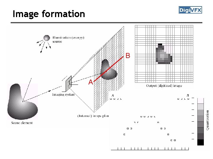
Image formation B A

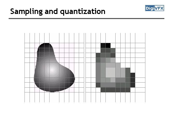
Sampling and quantization

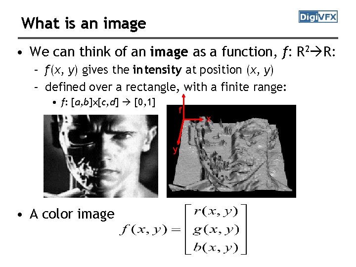
What is an image • We can think of an image as a function, f: R 2 R: – f(x, y) gives the intensity at position (x, y) – defined over a rectangle, with a finite range: • f: [a, b]x[c, d] [0, 1] f y • A color image x

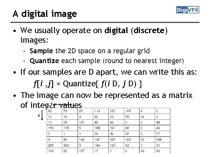
A digital image • We usually operate on digital (discrete) images: – Sample the 2 D space on a regular grid – Quantize each sample (round to nearest integer) • If our samples are D apart, we can write this as: f[i , j] = Quantize{ f(i D, j D) } • The image can now be represented as a matrix of integer values

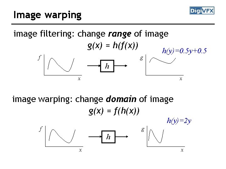
Image warping image filtering: change range of image g(x) = h(f(x)) f g h(y)=0. 5 y+0. 5 h x x image warping: change domain of image g(x) = f(h(x)) h(y)=2 y f g h x x

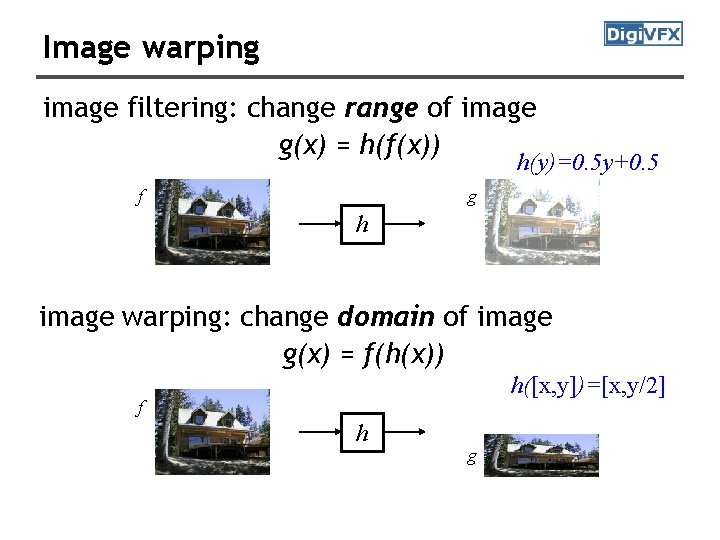
Image warping image filtering: change range of image g(x) = h(f(x)) h(y)=0. 5 y+0. 5 f g h image warping: change domain of image g(x) = f(h(x)) h([x, y])=[x, y/2] f h g

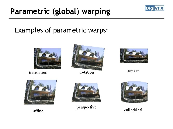
Parametric (global) warping Examples of parametric warps: translation affine rotation perspective aspect cylindrical

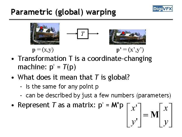
Parametric (global) warping T p = (x, y) p’ = (x’, y’) • Transformation T is a coordinate-changing machine: p’ = T(p) • What does it mean that T is global? – Is the same for any point p – can be described by just a few numbers (parameters) • Represent T as a matrix: p’ = M*p

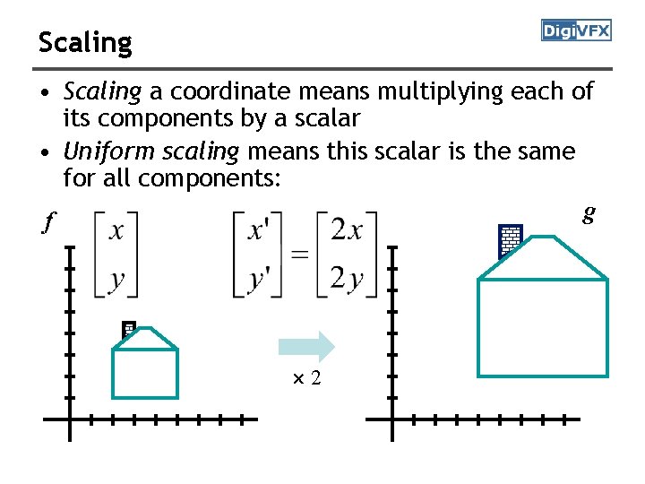
Scaling • Scaling a coordinate means multiplying each of its components by a scalar • Uniform scaling means this scalar is the same for all components: g f 2

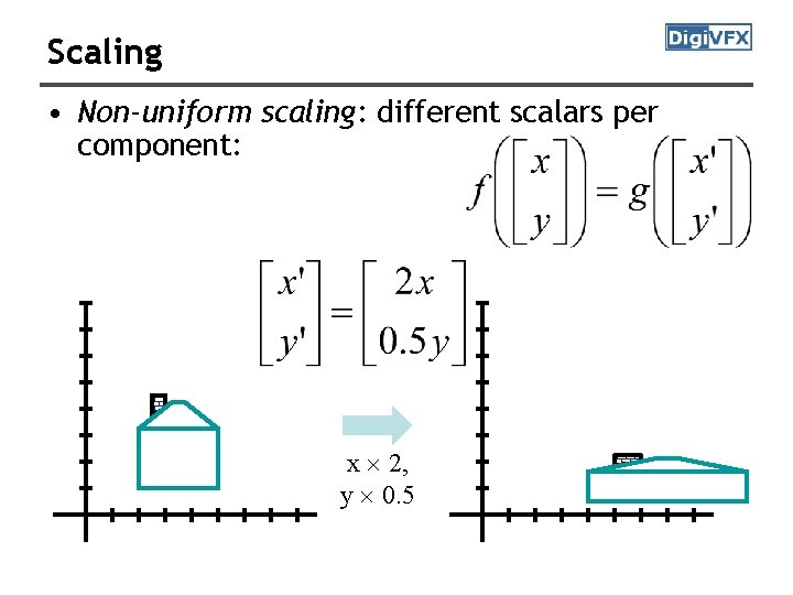
Scaling • Non-uniform scaling: different scalars per component: x 2, y 0. 5

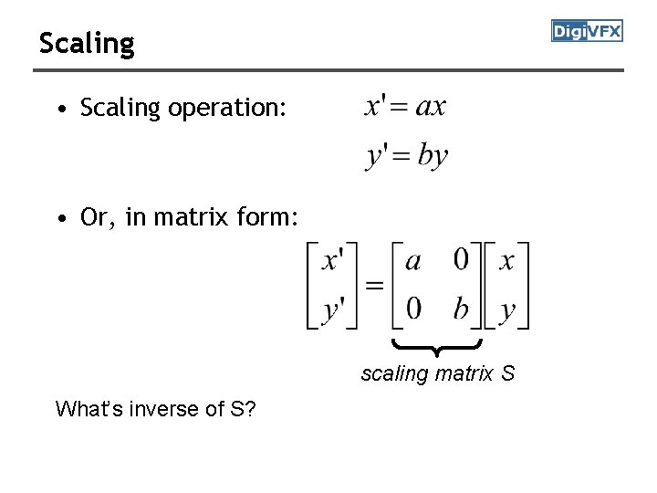
Scaling • Scaling operation: • Or, in matrix form: scaling matrix S What’s inverse of S?

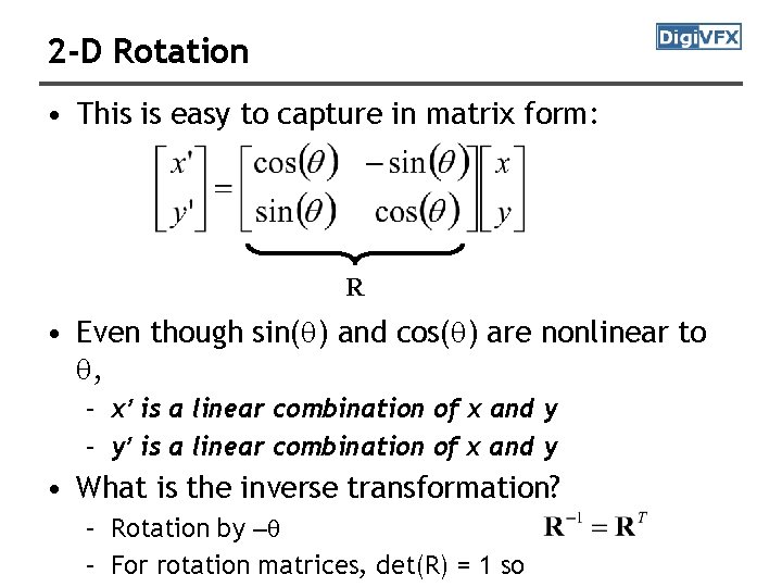
2 -D Rotation • This is easy to capture in matrix form: R • Even though sin(q) and cos(q) are nonlinear to q, – x’ is a linear combination of x and y – y’ is a linear combination of x and y • What is the inverse transformation? – Rotation by –q – For rotation matrices, det(R) = 1 so

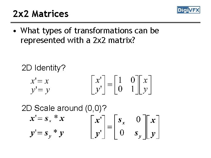
2 x 2 Matrices • What types of transformations can be represented with a 2 x 2 matrix? 2 D Identity? 2 D Scale around (0, 0)?

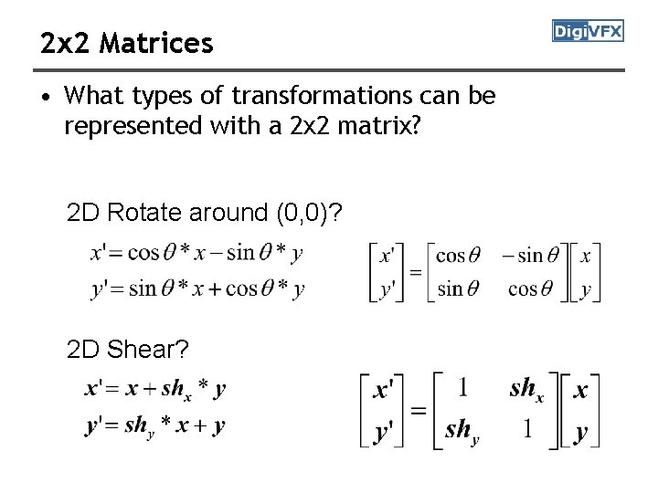
2 x 2 Matrices • What types of transformations can be represented with a 2 x 2 matrix? 2 D Rotate around (0, 0)? 2 D Shear?

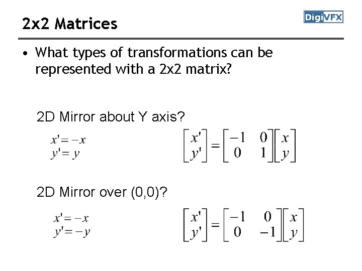
2 x 2 Matrices • What types of transformations can be represented with a 2 x 2 matrix? 2 D Mirror about Y axis? 2 D Mirror over (0, 0)?

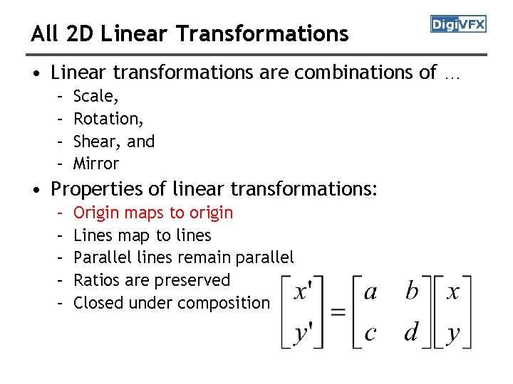
All 2 D Linear Transformations • Linear transformations are combinations of … – – Scale, Rotation, Shear, and Mirror • Properties of linear transformations: – – – Origin maps to origin Lines map to lines Parallel lines remain parallel Ratios are preserved Closed under composition

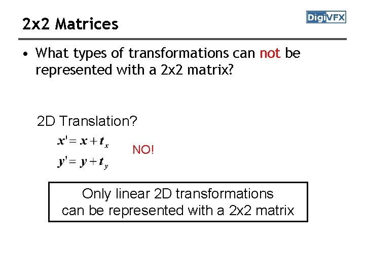
2 x 2 Matrices • What types of transformations can not be represented with a 2 x 2 matrix? 2 D Translation? NO! Only linear 2 D transformations can be represented with a 2 x 2 matrix

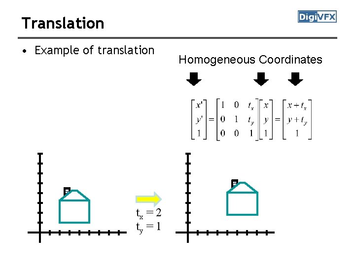
Translation • Example of translation tx = 2 ty = 1 Homogeneous Coordinates

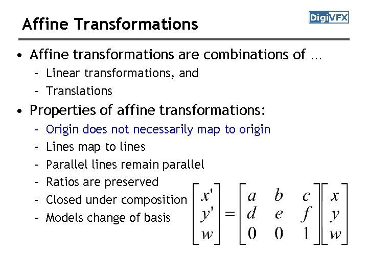
Affine Transformations • Affine transformations are combinations of … – Linear transformations, and – Translations • Properties of affine transformations: – – – Origin does not necessarily map to origin Lines map to lines Parallel lines remain parallel Ratios are preserved Closed under composition Models change of basis

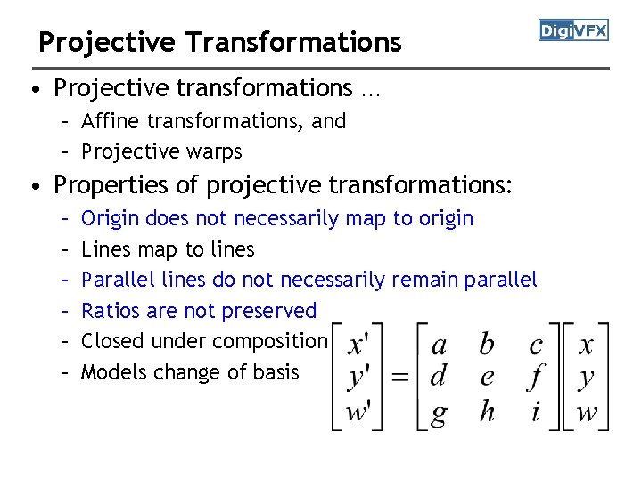
Projective Transformations • Projective transformations … – Affine transformations, and – Projective warps • Properties of projective transformations: – – – Origin does not necessarily map to origin Lines map to lines Parallel lines do not necessarily remain parallel Ratios are not preserved Closed under composition Models change of basis

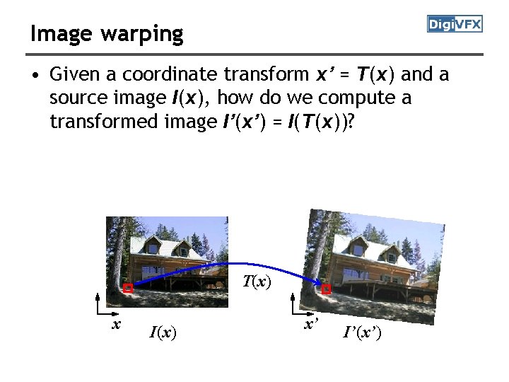
Image warping • Given a coordinate transform x’ = T(x) and a source image I(x), how do we compute a transformed image I’(x’) = I(T(x))? T(x) x I(x) x’ I’(x’)

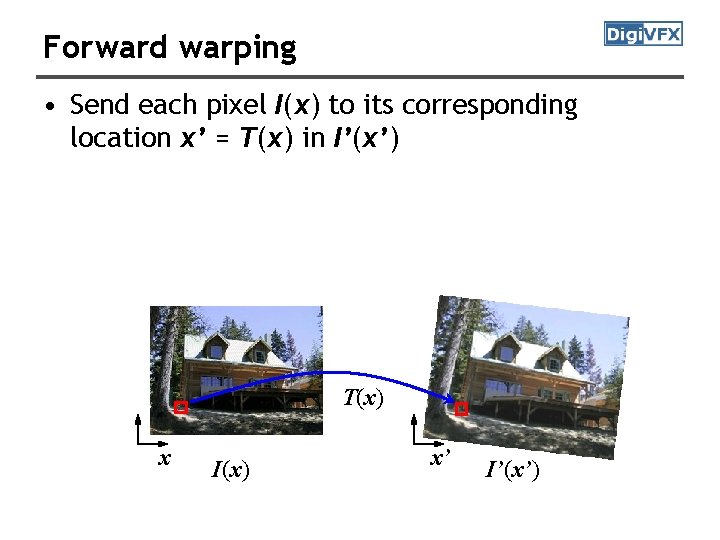
Forward warping • Send each pixel I(x) to its corresponding location x’ = T(x) in I’(x’) T(x) x I(x) x’ I’(x’)

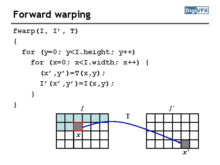
Forward warping fwarp(I, I’, T) { for (y=0; y<I. height; y++) for (x=0; x<I. width; x++) { (x’, y’)=T(x, y); I’(x’, y’)=I(x, y); } } I T I’ x x’

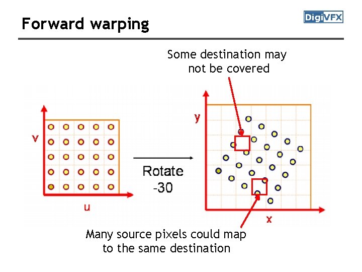
Forward warping Some destination may not be covered Many source pixels could map to the same destination

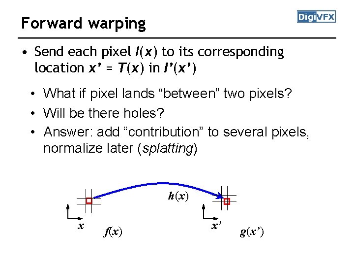
Forward warping • Send each pixel I(x) to its corresponding location x’ = T(x) in I’(x’) • What if pixel lands “between” two pixels? • Will be there holes? • Answer: add “contribution” to several pixels, normalize later (splatting) h(x) x f(x) x’ g(x’)

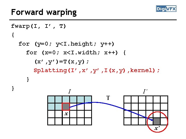
Forward warping fwarp(I, I’, T) { for (y=0; y<I. height; y++) for (x=0; x<I. width; x++) { (x’, y’)=T(x, y); Splatting(I’, x’, y’, I(x, y), kernel); } } I I’ T x x’

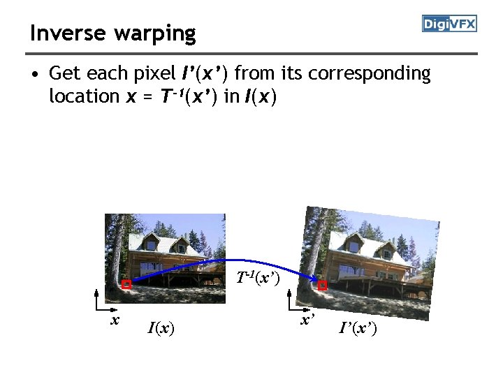
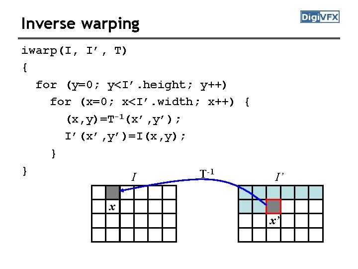
Inverse warping • Get each pixel I’(x’) from its corresponding location x = T-1(x’) in I(x) T-1(x’) x I(x) x’ I’(x’)

Inverse warping iwarp(I, I’, T) { for (y=0; y<I’. height; y++) for (x=0; x<I’. width; x++) { (x, y)=T-1(x’, y’); I’(x’, y’)=I(x, y); } } T-1 I I’ x x’

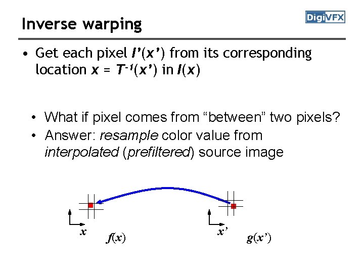
Inverse warping • Get each pixel I’(x’) from its corresponding location x = T-1(x’) in I(x) • What if pixel comes from “between” two pixels? • Answer: resample color value from interpolated (prefiltered) source image x f(x) x’ g(x’)

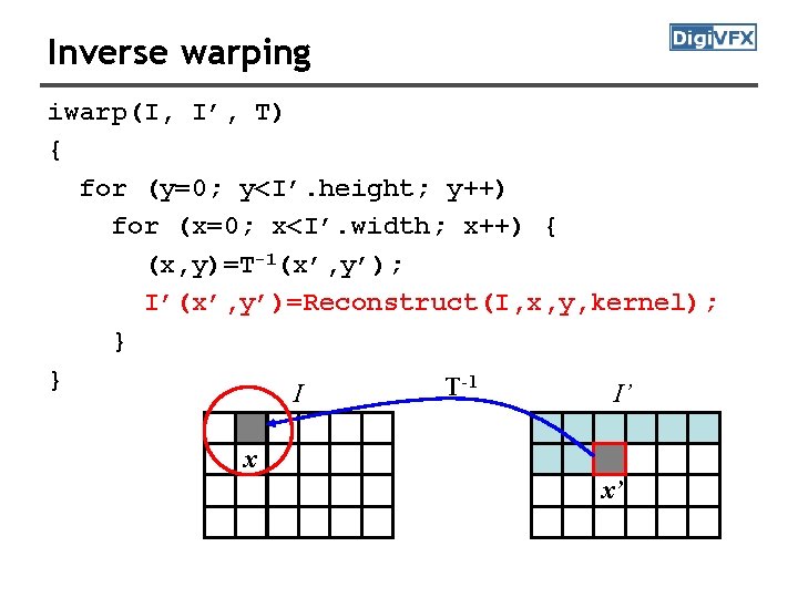
Inverse warping iwarp(I, I’, T) { for (y=0; y<I’. height; y++) for (x=0; x<I’. width; x++) { (x, y)=T-1(x’, y’); I’(x’, y’)=Reconstruct(I, x, y, kernel); } } T-1 I I’ x x’

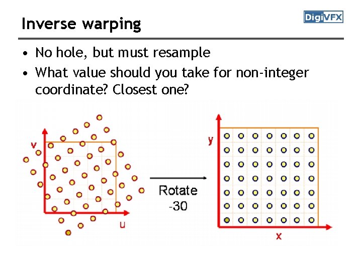
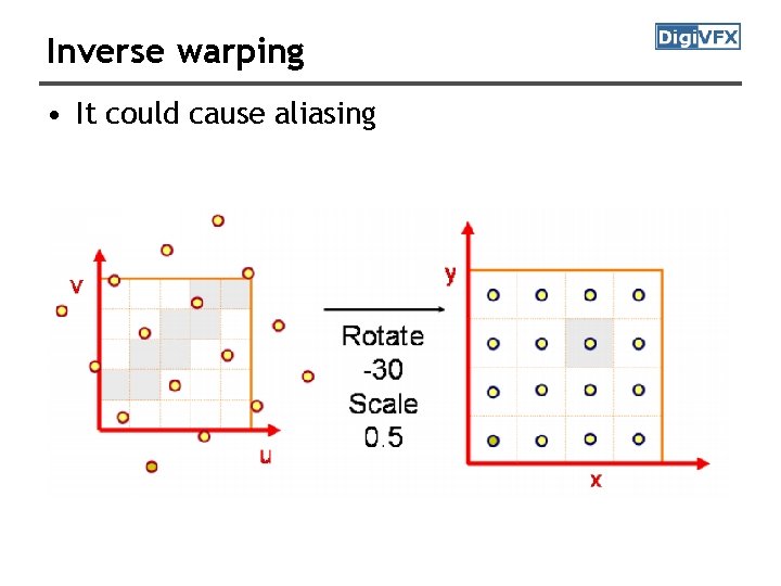
Inverse warping • No hole, but must resample • What value should you take for non-integer coordinate? Closest one?

Inverse warping • It could cause aliasing

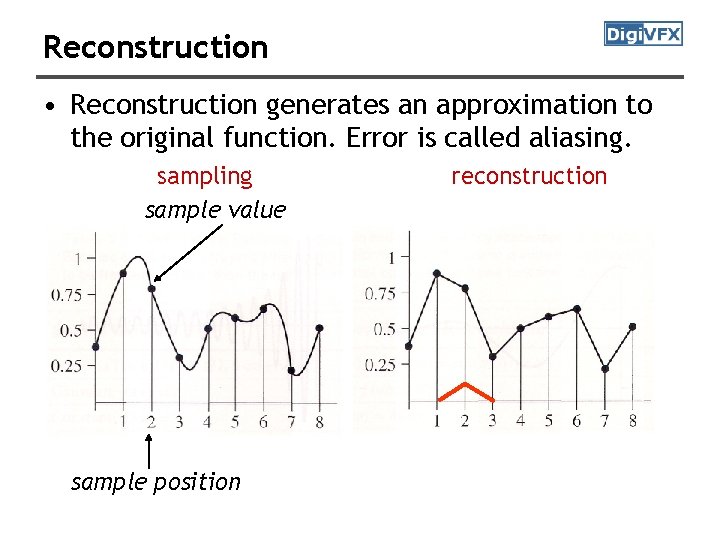
Reconstruction • Reconstruction generates an approximation to the original function. Error is called aliasing. sampling sample value sample position reconstruction

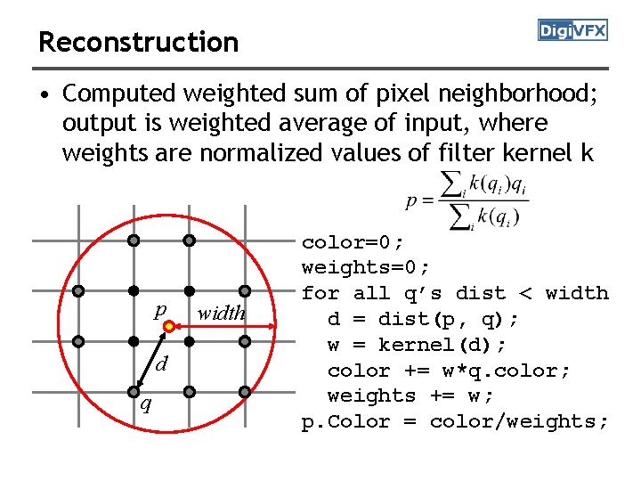
Reconstruction • Computed weighted sum of pixel neighborhood; output is weighted average of input, where weights are normalized values of filter kernel k p d q width color=0; weights=0; for all q’s dist < width d = dist(p, q); w = kernel(d); color += w*q. color; weights += w; p. Color = color/weights;

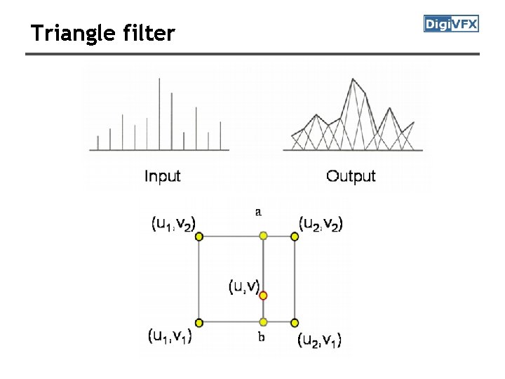
Triangle filter

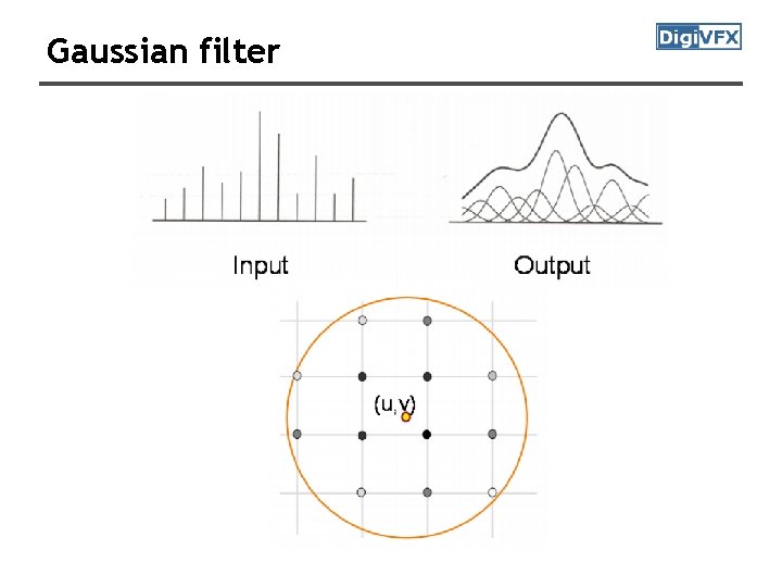
Gaussian filter

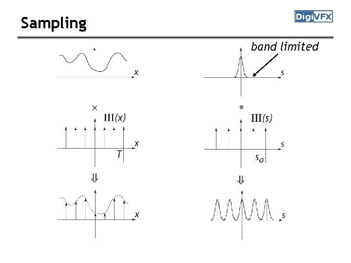
Sampling band limited

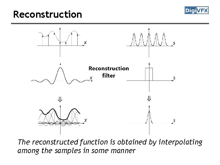
Reconstruction The reconstructed function is obtained by interpolating among the samples in some manner

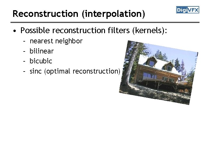
Reconstruction (interpolation) • Possible reconstruction filters (kernels): – – nearest neighbor bilinear bicubic sinc (optimal reconstruction)

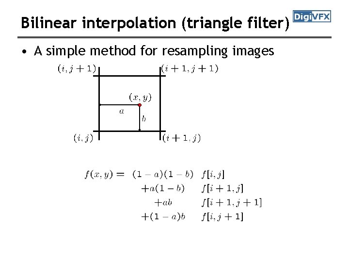
Bilinear interpolation (triangle filter) • A simple method for resampling images

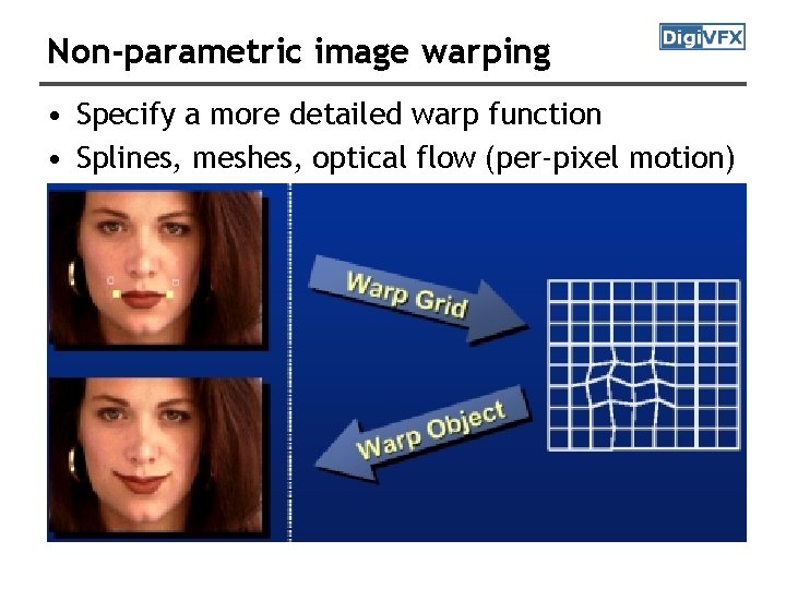
Non-parametric image warping • Specify a more detailed warp function • Splines, meshes, optical flow (per-pixel motion)

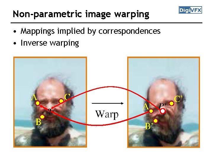
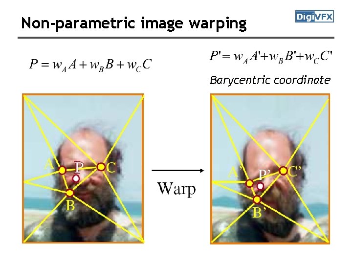
Non-parametric image warping • Mappings implied by correspondences • Inverse warping ? P’

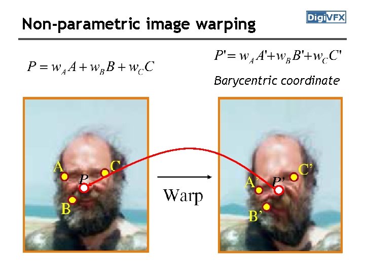
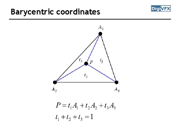
Non-parametric image warping Barycentric coordinate P P’

Barycentric coordinates

Non-parametric image warping Barycentric coordinate

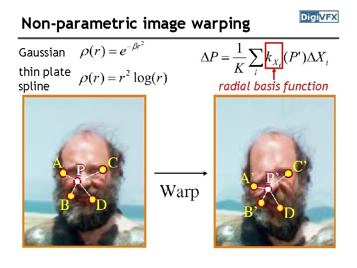
Non-parametric image warping Gaussian thin plate spline radial basis function

Image warping • Warping is a useful operation for mosaics, video matching, view interpolation and so on.

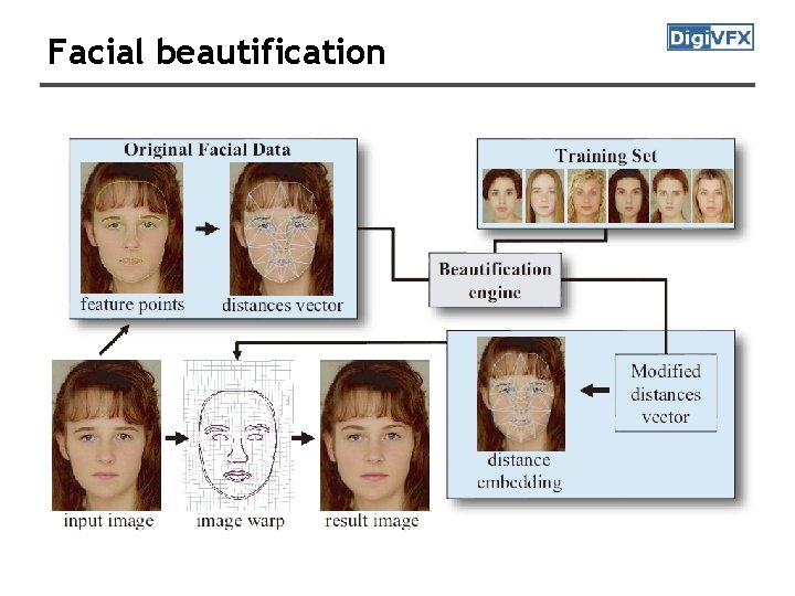
An application of image warping: face beautification

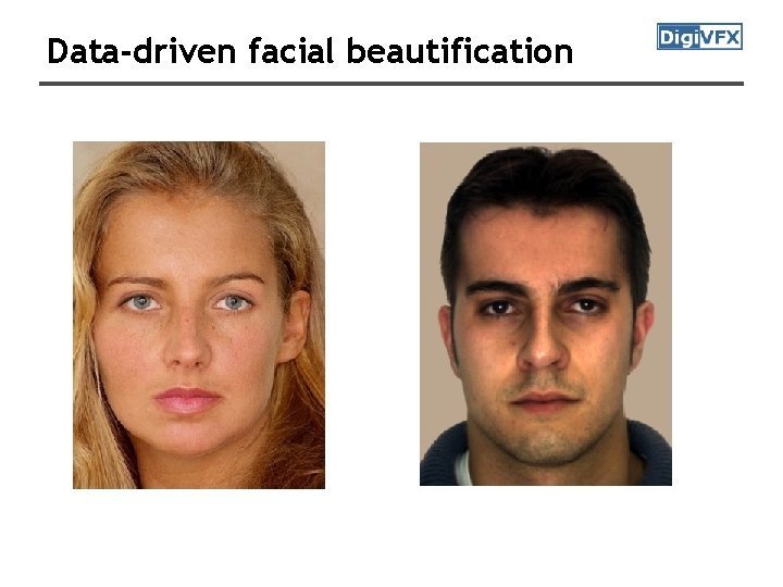
Data-driven facial beautification

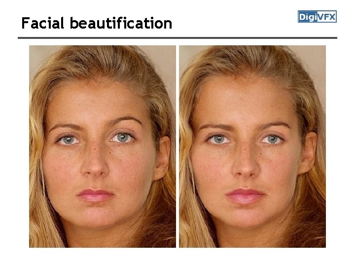
Facial beautification

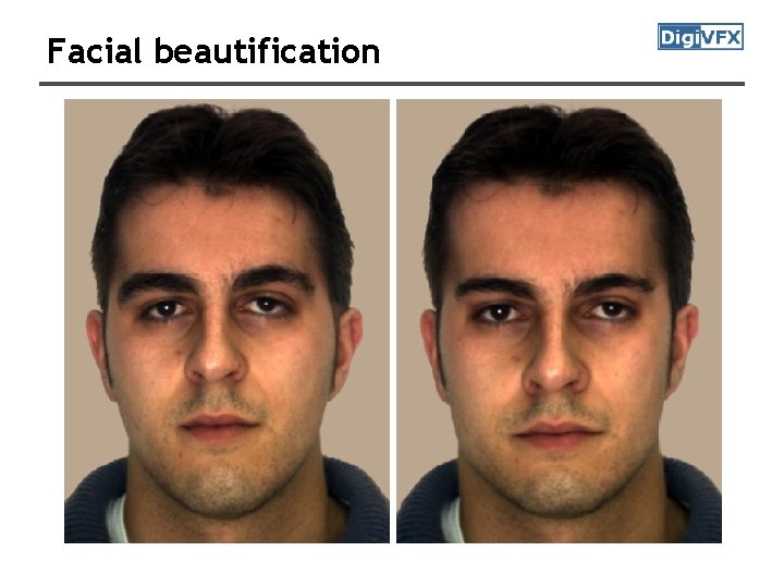
Facial beautification

Facial beautification

Training set • Face images – 92 young Caucasian female – 33 young Caucasian male

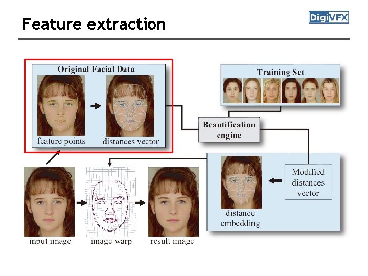
Feature extraction

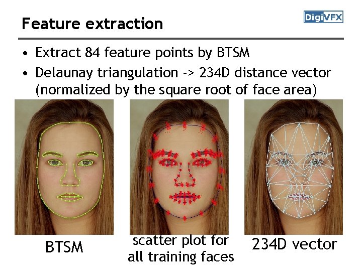
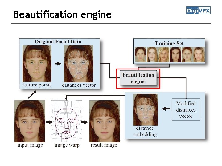
Feature extraction • Extract 84 feature points by BTSM • Delaunay triangulation -> 234 D distance vector (normalized by the square root of face area) BTSM scatter plot for all training faces 234 D vector

Beautification engine

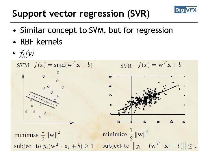
Support vector regression (SVR) • Similar concept to SVM, but for regression • RBF kernels • fb(v)

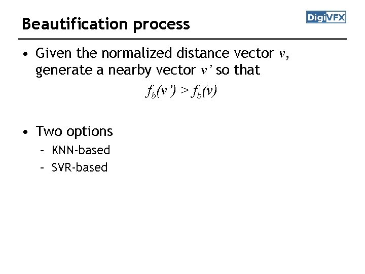
Beautification process • Given the normalized distance vector v, generate a nearby vector v’ so that fb(v’) > fb(v) • Two options – KNN-based – SVR-based

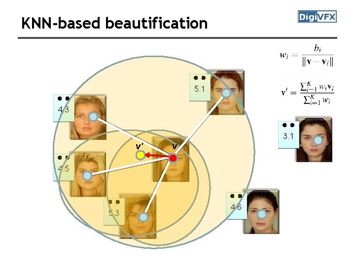
KNN-based beautification 5. 1 4. 3 3. 1 v' v 4. 5 5. 3 4. 6

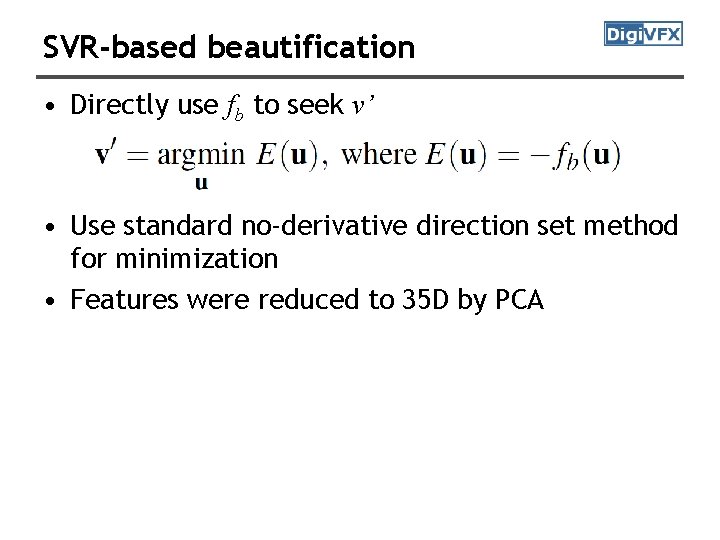
SVR-based beautification • Directly use fb to seek v’ • Use standard no-derivative direction set method for minimization • Features were reduced to 35 D by PCA

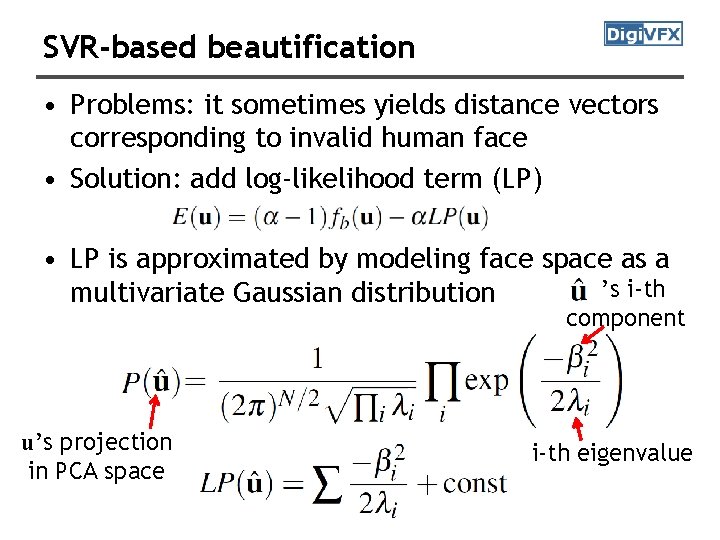
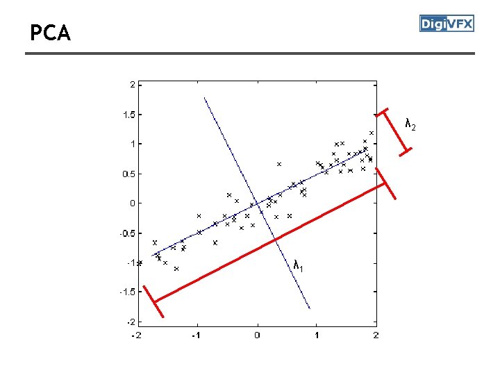
SVR-based beautification • Problems: it sometimes yields distance vectors corresponding to invalid human face • Solution: add log-likelihood term (LP) • LP is approximated by modeling face space as a ’s i-th multivariate Gaussian distribution component u’s projection in PCA space i-th eigenvalue

PCA λ 2 λ 1

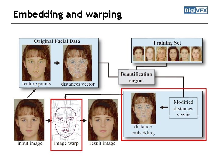
Embedding and warping

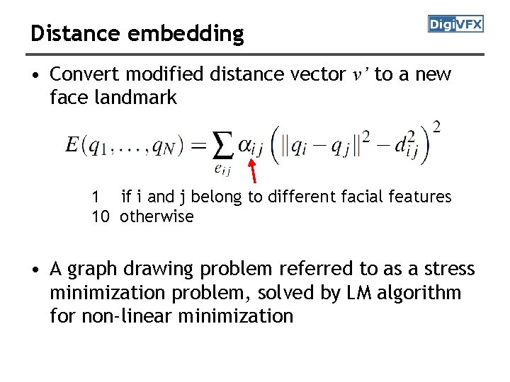
Distance embedding • Convert modified distance vector v’ to a new face landmark 1 if i and j belong to different facial features 10 otherwise • A graph drawing problem referred to as a stress minimization problem, solved by LM algorithm for non-linear minimization

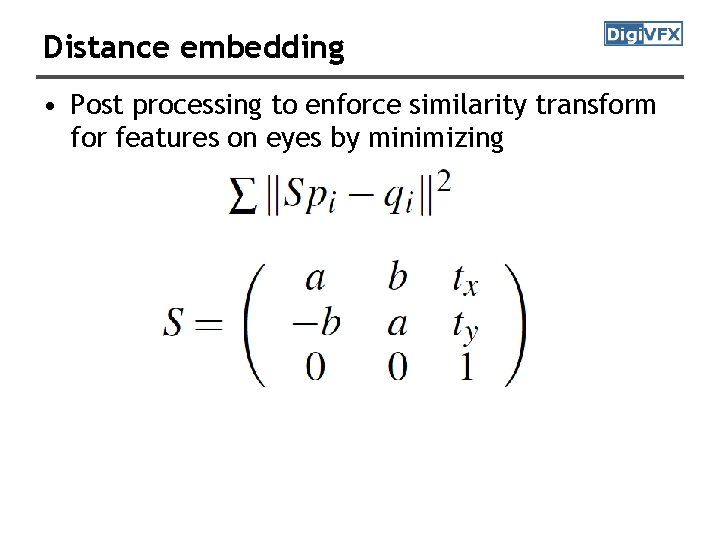
Distance embedding • Post processing to enforce similarity transform for features on eyes by minimizing

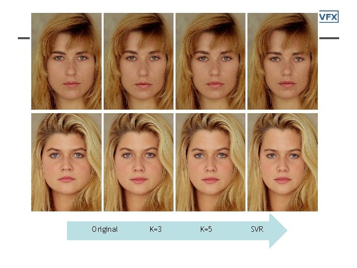
Original K=3 K=5 SVR

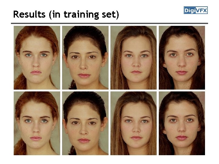
Results (in training set)

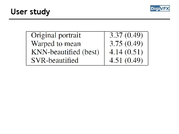
User study

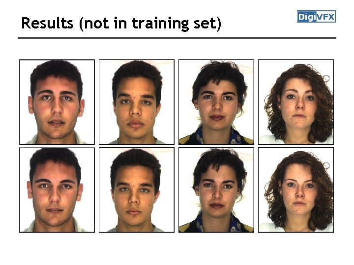
Results (not in training set)

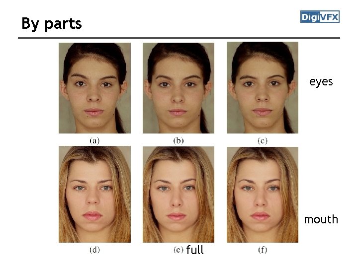
By parts eyes mouth full

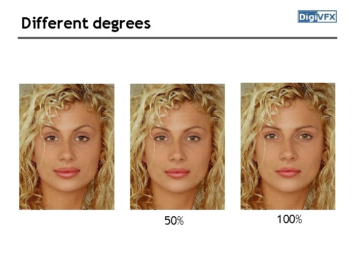
Different degrees 50% 100%

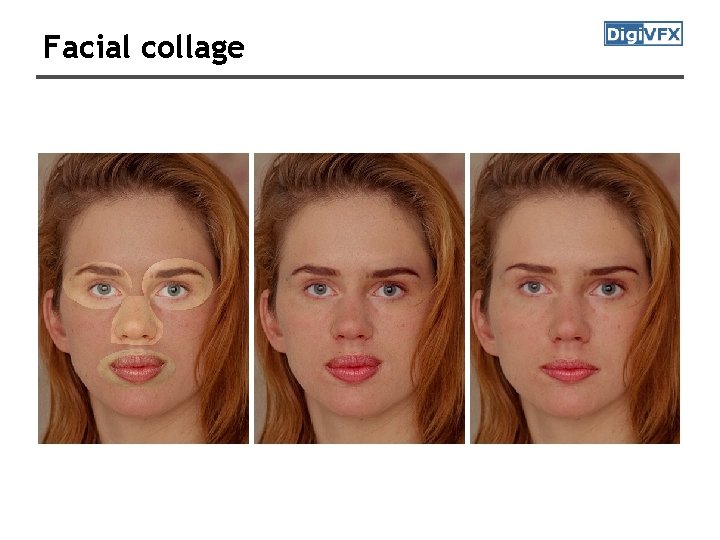
Facial collage

Results • video

Image morphing

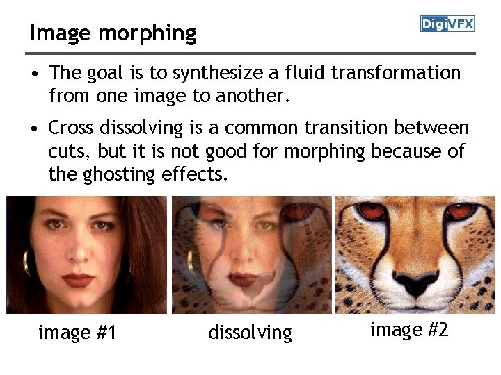
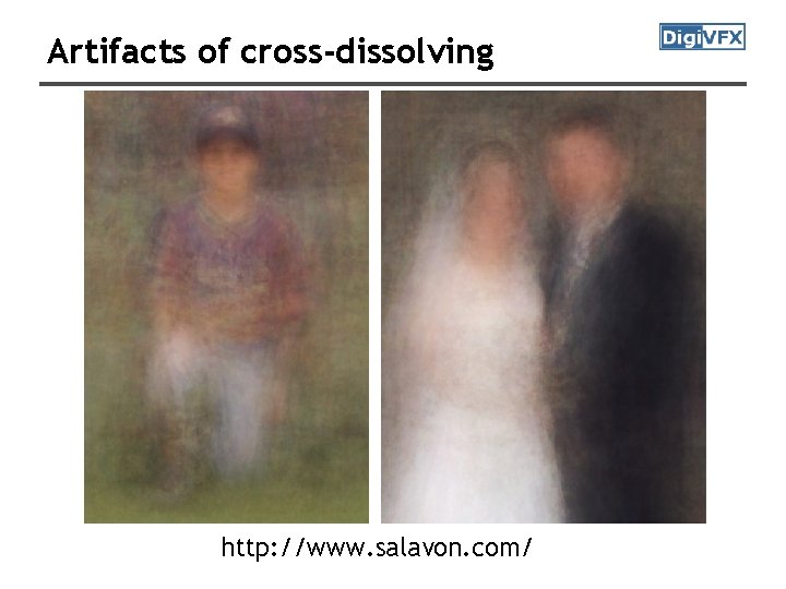
Image morphing • The goal is to synthesize a fluid transformation from one image to another. • Cross dissolving is a common transition between cuts, but it is not good for morphing because of the ghosting effects. image #1 dissolving image #2

Artifacts of cross-dissolving http: //www. salavon. com/

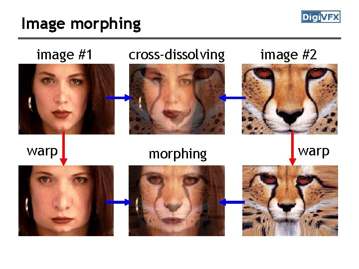
Image morphing • Why ghosting? • Morphing = warping + cross-dissolving shape (geometric) color (photometric)

Image morphing image #1 warp cross-dissolving morphing image #2 warp

Morphing sequence

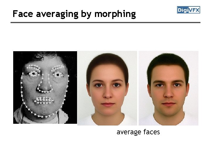
Face averaging by morphing average faces

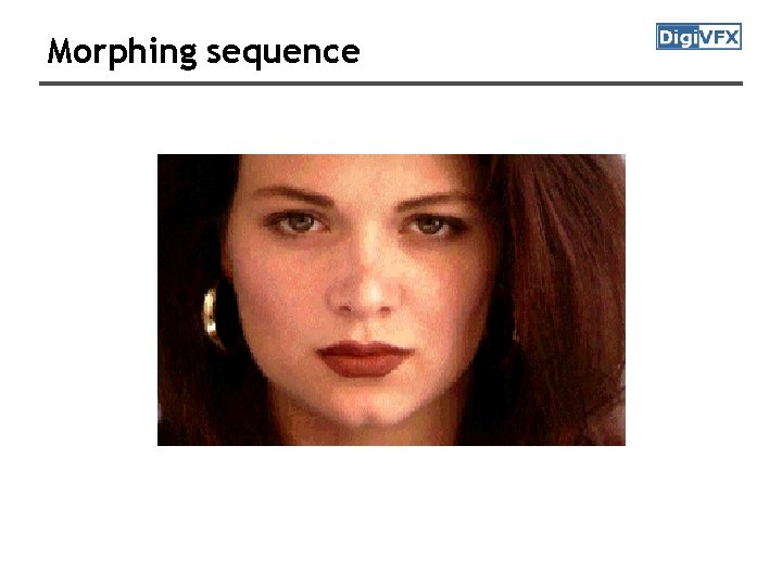
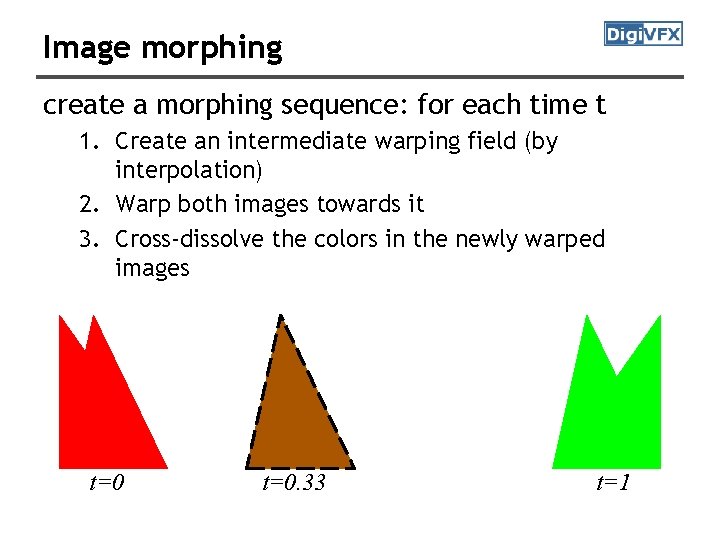
Image morphing create a morphing sequence: for each time t 1. Create an intermediate warping field (by interpolation) 2. Warp both images towards it 3. Cross-dissolve the colors in the newly warped images t=0. 33 t=1

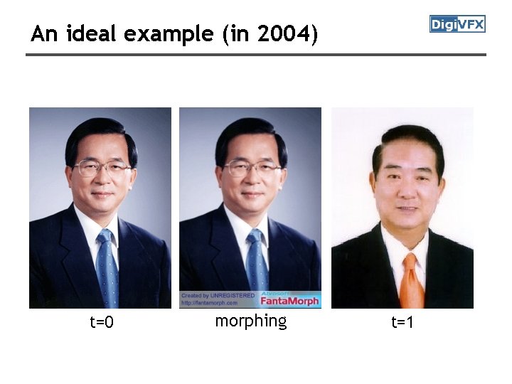
An ideal example (in 2004) t=0 morphing t=0. 25 t=0. 75 t=1

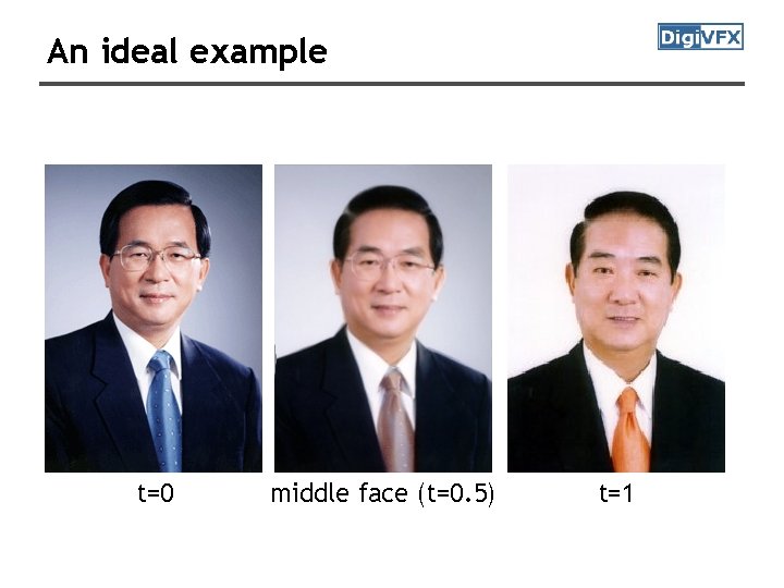
An ideal example t=0 middle face (t=0. 5) t=1

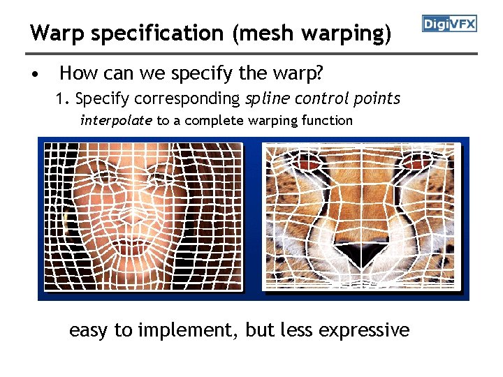
Warp specification (mesh warping) • How can we specify the warp? 1. Specify corresponding spline control points interpolate to a complete warping function easy to implement, but less expressive

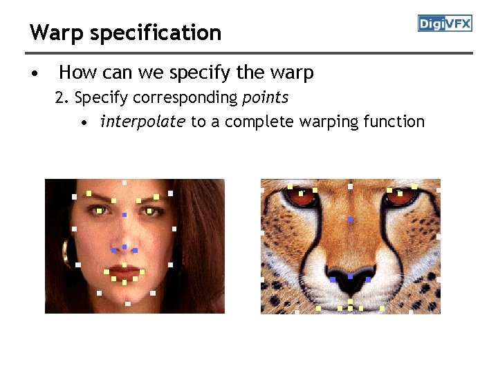
Warp specification • How can we specify the warp 2. Specify corresponding points • interpolate to a complete warping function

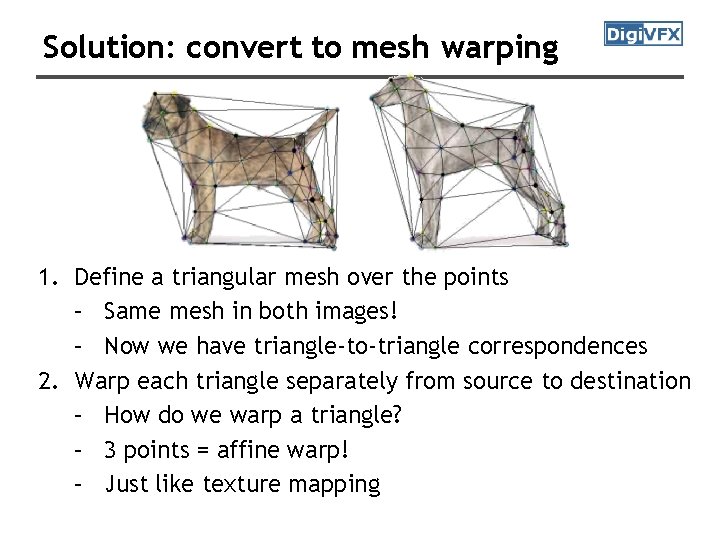
Solution: convert to mesh warping 1. Define a triangular mesh over the points – Same mesh in both images! – Now we have triangle-to-triangle correspondences 2. Warp each triangle separately from source to destination – How do we warp a triangle? – 3 points = affine warp! – Just like texture mapping

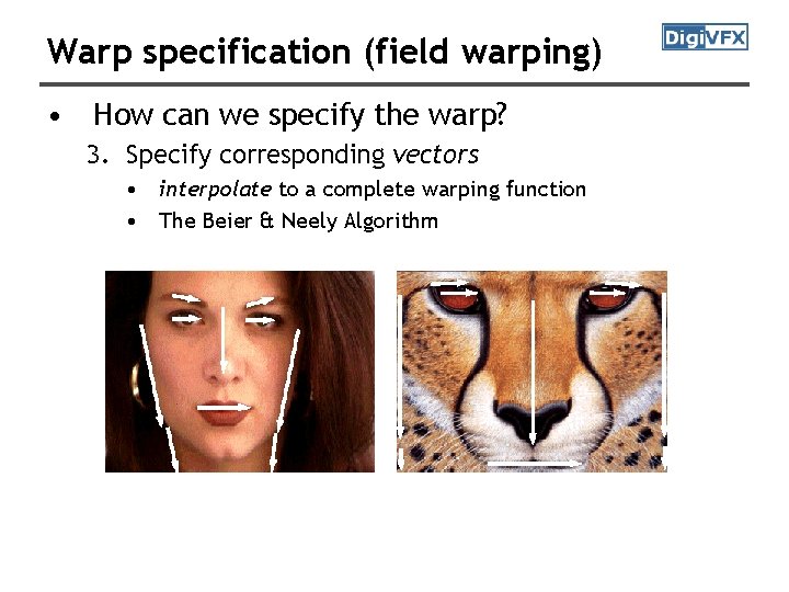
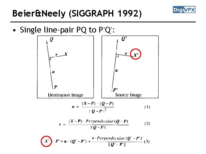
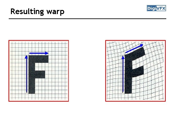
Warp specification (field warping) • How can we specify the warp? 3. Specify corresponding vectors • interpolate to a complete warping function • The Beier & Neely Algorithm

Beier&Neely (SIGGRAPH 1992) • Single line-pair PQ to P’Q’:

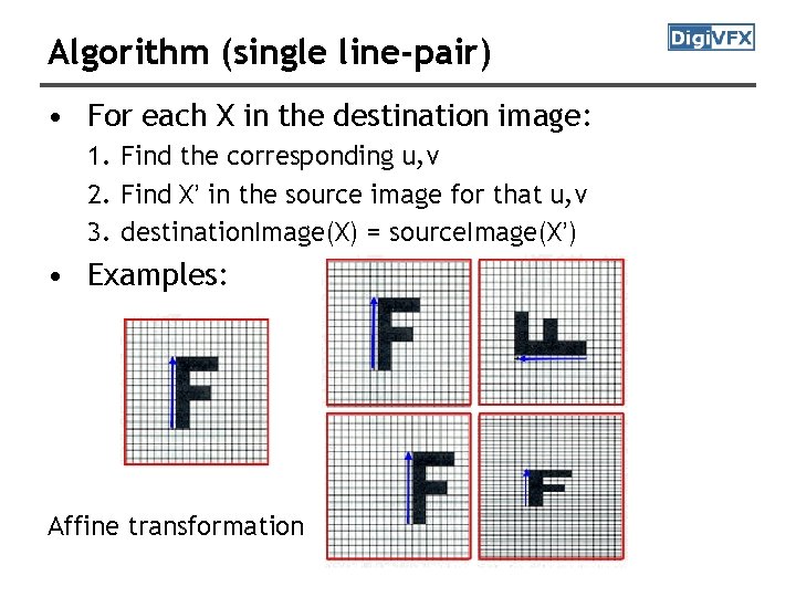
Algorithm (single line-pair) • For each X in the destination image: 1. Find the corresponding u, v 2. Find X’ in the source image for that u, v 3. destination. Image(X) = source. Image(X’) • Examples: Affine transformation

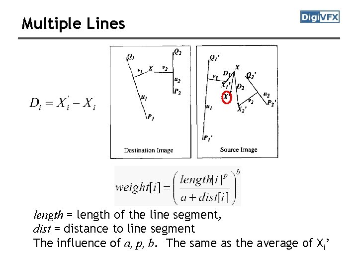
Multiple Lines length = length of the line segment, dist = distance to line segment The influence of a, p, b. The same as the average of Xi’

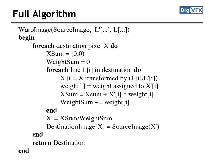
Full Algorithm

Resulting warp

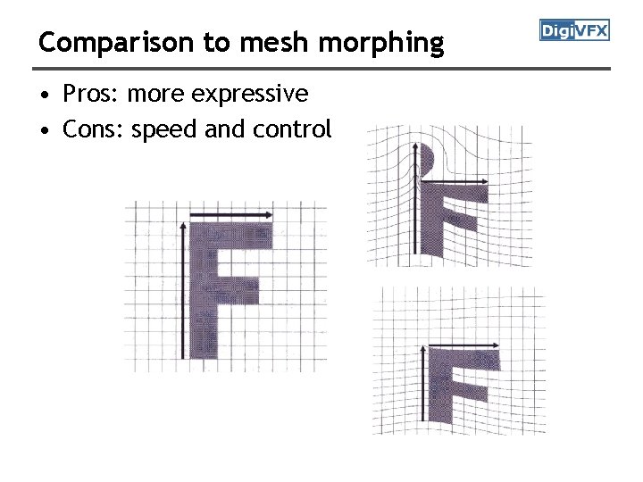
Comparison to mesh morphing • Pros: more expressive • Cons: speed and control

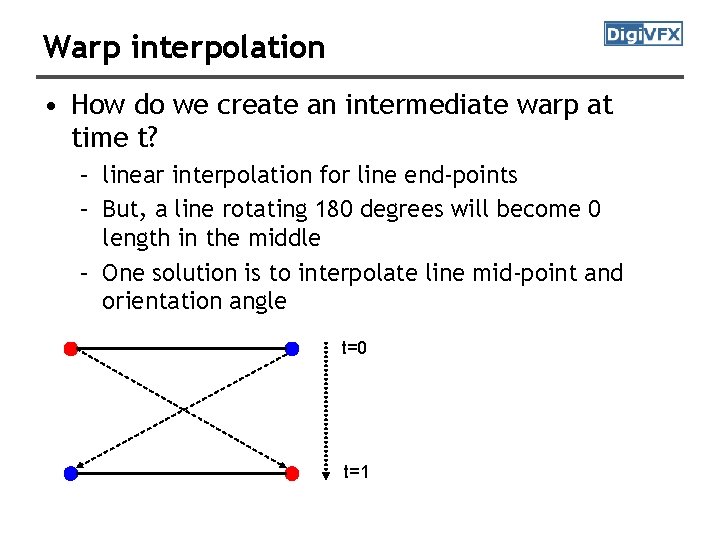
Warp interpolation • How do we create an intermediate warp at time t? – linear interpolation for line end-points – But, a line rotating 180 degrees will become 0 length in the middle – One solution is to interpolate line mid-point and orientation angle t=0 t=1

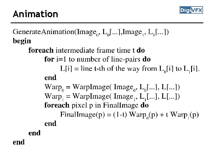
Animation

Animated sequences • Specify keyframes and interpolate the lines for the inbetween frames • Require a lot of tweaking

Results Michael Jackson’s MTV “Black or White”

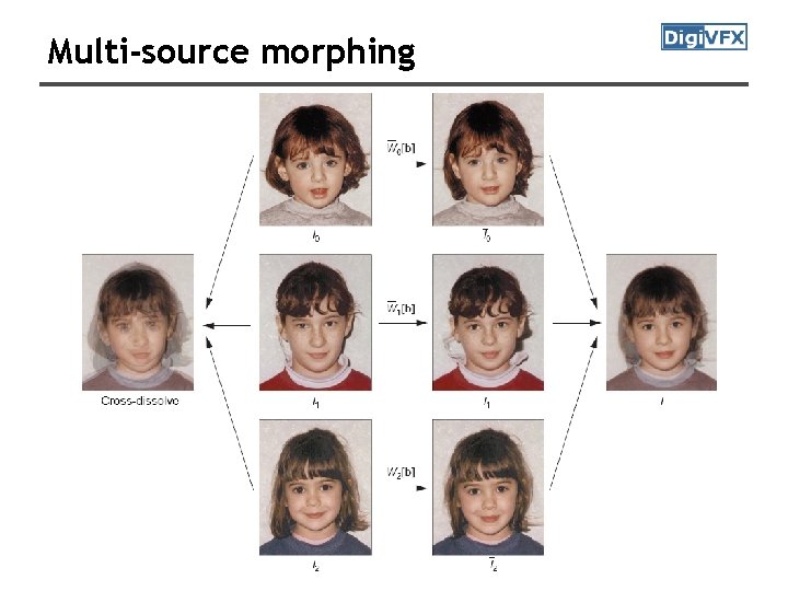
Multi-source morphing

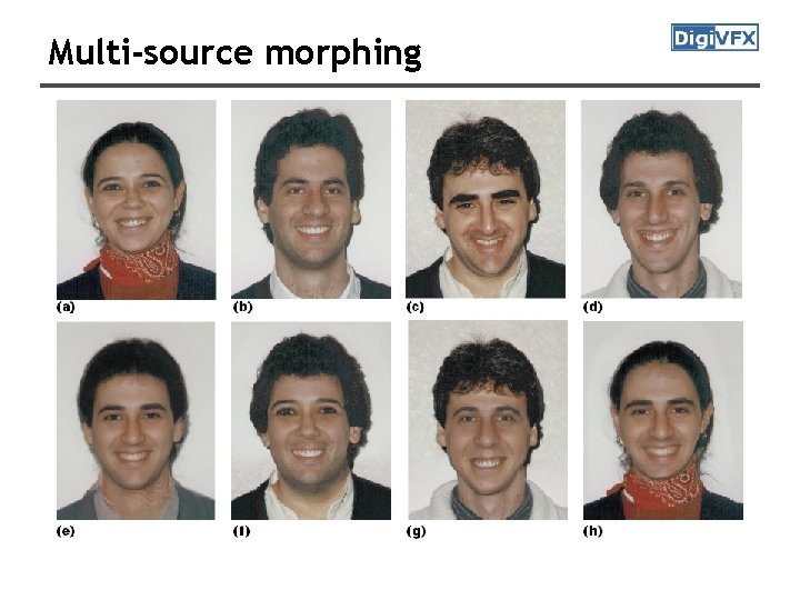
Multi-source morphing

References • Thaddeus Beier, Shawn Neely, Feature-Based Image Metamorphosis, SIGGRAPH 1992, pp 35 -42. • Detlef Ruprecht, Heinrich Muller, Image Warping with Scattered Data Interpolation, IEEE Computer Graphics and Applications, March 1995, pp 37 -43. • Seung-Yong Lee, Kyung-Yong Chwa, Sung Yong Shin, Image Metamorphosis Using Snakes and Free-Form Deformations, SIGGRAPH 1995. • Seungyong Lee, Wolberg, G. , Sung Yong Shin, Polymorph: morphing among multiple images, IEEE Computer Graphics and Applications, Vol. 18, No. 1, 1998, pp 58 -71. • Peinsheng Gao, Thomas Sederberg, A work minimization approach to image morphing, The Visual Computer, 1998, pp 390 -400. • George Wolberg, Image morphing: a survey, The Visual Computer, 1998, pp 360 -372. • Data-Driven Enhancement of Facial Attractiveness, SIGGRAPH 2008

Project #1: image morphing

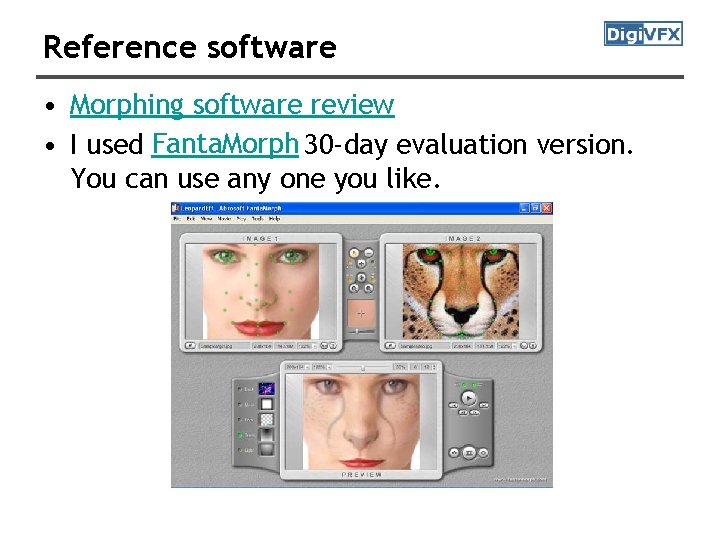
Reference software • Morphing software review • I used Fanta. Morph 30 -day evaluation version. You can use any one you like.

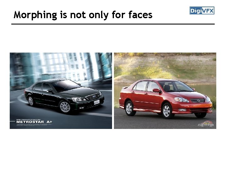
Morphing is not only for faces

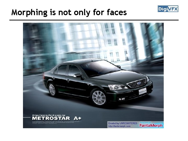
Morphing is not only for faces