Sampling and Reconstruction Digital Image Synthesis YungYu Chuang

Sampling and Reconstruction Digital Image Synthesis Yung-Yu Chuang 10/29/2009 with slides by Pat Hanrahan, Torsten Moller and Brian Curless

Sampling theory • Sampling theory: theory of taking discrete sample values (grid of color pixels) from functions defined over continuous domains (incident radiance defined over the film plane) and then using those samples to reconstruct new functions that are similar to the original (reconstruction). Sampler: selects sample points on the image plane Filter: blends multiple samples together

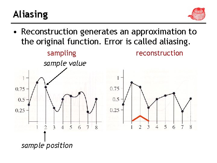
Aliasing • Reconstruction generates an approximation to the original function. Error is called aliasing. sampling sample value sample position reconstruction

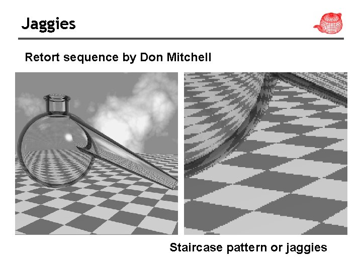
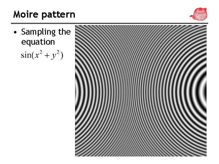
Sampling in computer graphics • Artifacts due to sampling - Aliasing – – – Jaggies Moire Flickering small objects Sparkling highlights Temporal strobing (such as Wagon-wheel effect) • Preventing these artifacts - Antialiasing

Jaggies Retort sequence by Don Mitchell Staircase pattern or jaggies

Moire pattern • Sampling the equation

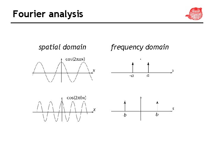
Fourier analysis • Can be used to evaluate the quality between the reconstruction and the original. • The concept was introduced to Graphics by Robert Cook in 1986. (extended by Don Rob Cook Mitchell) V. P. of Pixar 1981 M. S. Cornell 1987 SIGGRAPH Achievement award 1999 Fellow of ACM 2001 Academic Award with Ed Catmull and Loren Carpenter (for Renderman)

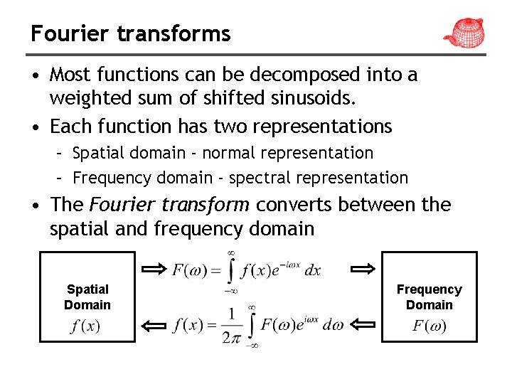
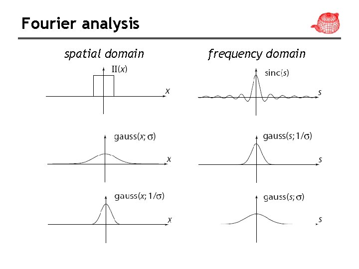
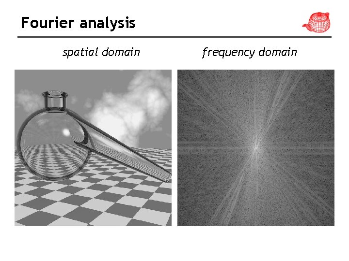
Fourier transforms • Most functions can be decomposed into a weighted sum of shifted sinusoids. • Each function has two representations – Spatial domain - normal representation – Frequency domain - spectral representation • The Fourier transform converts between the spatial and frequency domain Spatial Domain Frequency Domain

Fourier analysis spatial domain frequency domain

Fourier analysis spatial domain frequency domain

Fourier analysis spatial domain frequency domain

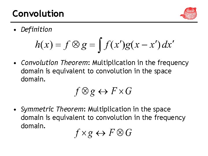
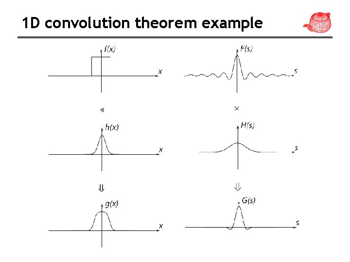
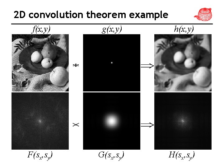
Convolution • Definition • Convolution Theorem: Multiplication in the frequency domain is equivalent to convolution in the space domain. • Symmetric Theorem: Multiplication in the space domain is equivalent to convolution in the frequency domain.

1 D convolution theorem example

2 D convolution theorem example f(x, y) g(x, y) h(x, y) F(sx, sy) G(sx, sy) H(sx, sy)

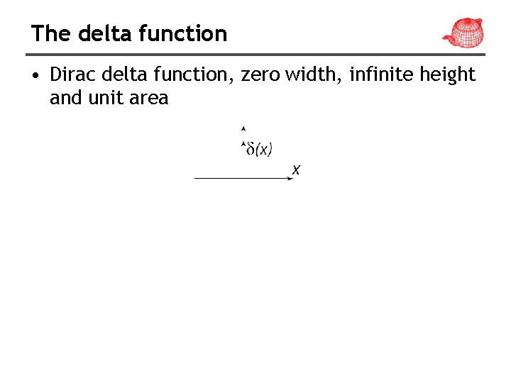
The delta function • Dirac delta function, zero width, infinite height and unit area

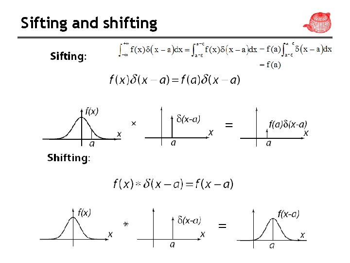
Sifting and shifting

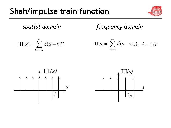
Shah/impulse train function spatial domain frequency domain ,

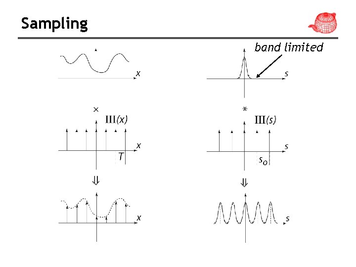
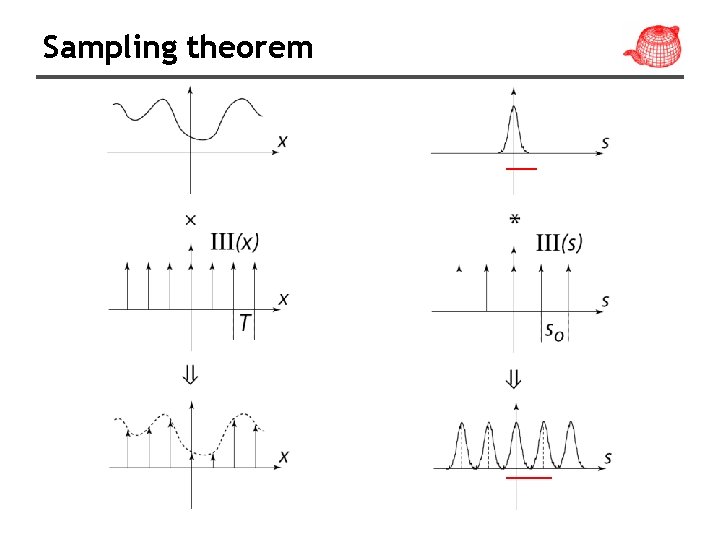
Sampling band limited

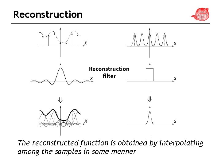
Reconstruction The reconstructed function is obtained by interpolating among the samples in some manner

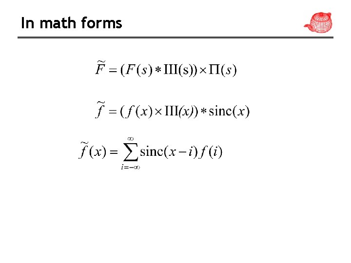
In math forms

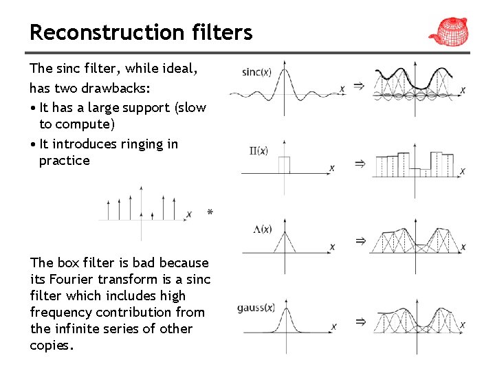
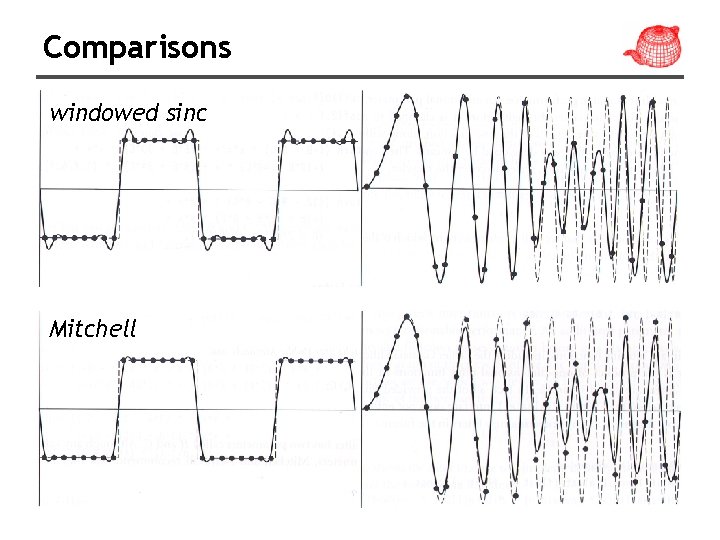
Reconstruction filters The sinc filter, while ideal, has two drawbacks: • It has a large support (slow to compute) • It introduces ringing in practice The box filter is bad because its Fourier transform is a sinc filter which includes high frequency contribution from the infinite series of other copies.

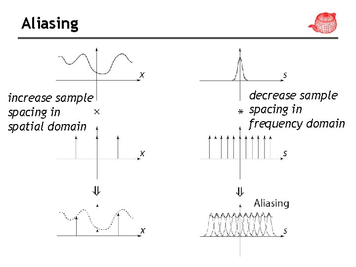
Aliasing increase sample spacing in spatial domain decrease sample spacing in frequency domain

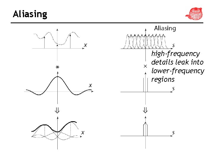
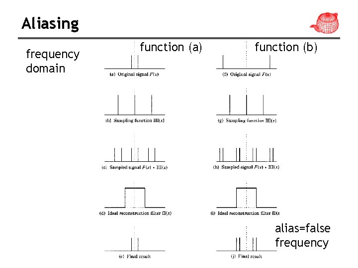
Aliasing high-frequency details leak into lower-frequency regions

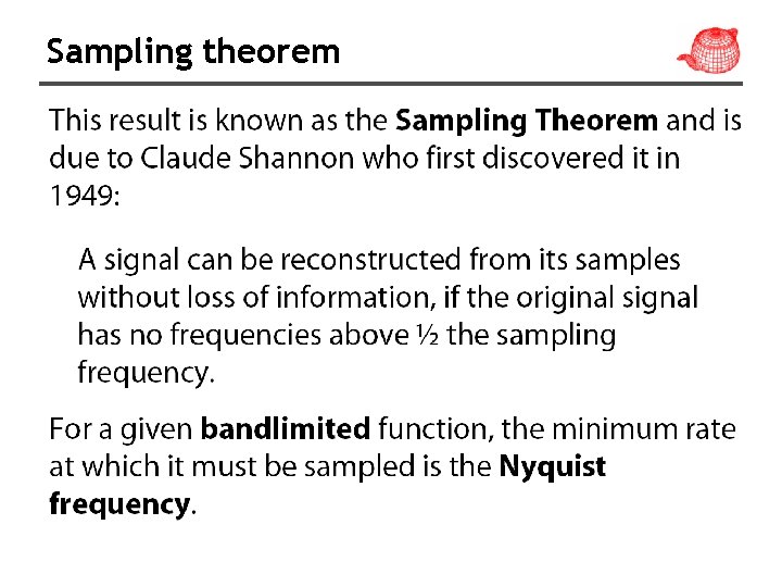
Sampling theorem

Sampling theorem

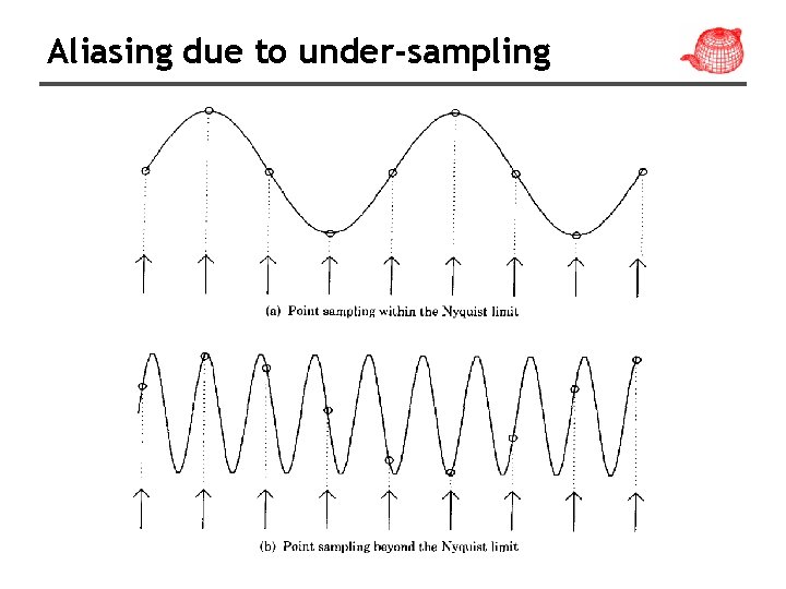
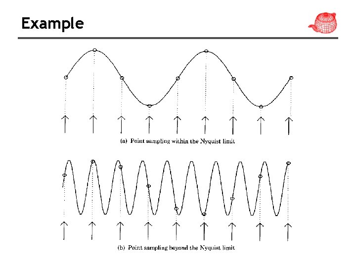
Aliasing due to under-sampling

Sampling theorem • For band limited functions, we can just increase the sampling rate • However, few of interesting functions in computer graphics are band limited, in particular, functions with discontinuities. • It is mostly because the discontinuity always falls between two samples and the samples provides no information about this discontinuity.

Aliasing • Prealiasing: due to sampling under Nyquist rate • Postaliasing: due to use of imperfect reconstruction filter

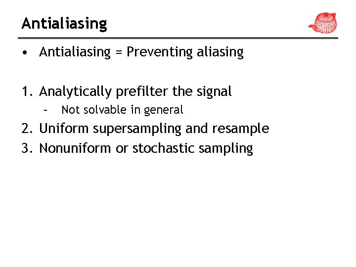
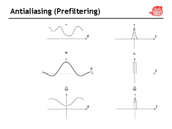
Antialiasing • Antialiasing = Preventing aliasing 1. Analytically prefilter the signal – Not solvable in general 2. Uniform supersampling and resample 3. Nonuniform or stochastic sampling

Antialiasing (Prefiltering)

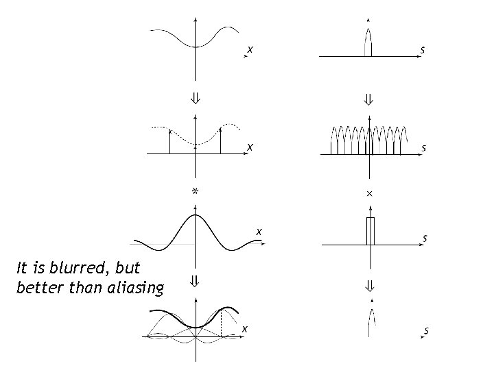
It is blurred, but better than aliasing

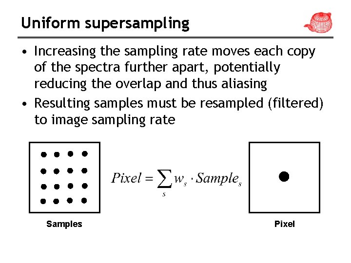
Uniform supersampling • Increasing the sampling rate moves each copy of the spectra further apart, potentially reducing the overlap and thus aliasing • Resulting samples must be resampled (filtered) to image sampling rate Samples Pixel

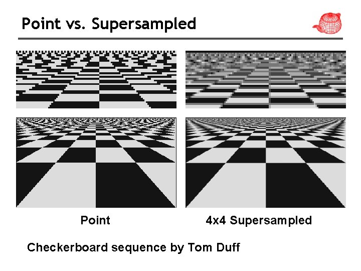
Point vs. Supersampled Point 4 x 4 Supersampled Checkerboard sequence by Tom Duff

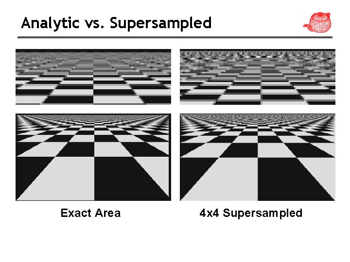
Analytic vs. Supersampled Exact Area 4 x 4 Supersampled

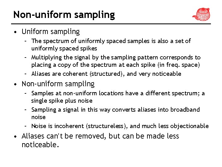
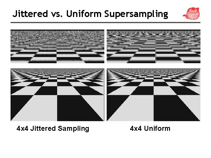
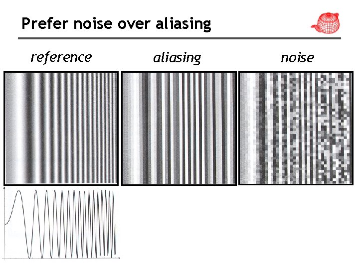
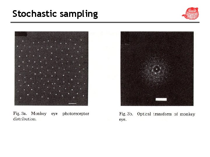
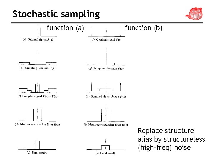
Non-uniform sampling • Uniform sampling – The spectrum of uniformly spaced samples is also a set of uniformly spaced spikes – Multiplying the signal by the sampling pattern corresponds to placing a copy of the spectrum at each spike (in freq. space) – Aliases are coherent (structured), and very noticeable • Non-uniform sampling – Samples at non-uniform locations have a different spectrum; a single spike plus noise – Sampling a signal in this way converts aliases into broadband noise – Noise is incoherent (structureless), and much less objectionable • Aliases can’t be removed, but can be made less noticeable.

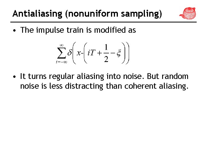
Antialiasing (nonuniform sampling) • The impulse train is modified as • It turns regular aliasing into noise. But random noise is less distracting than coherent aliasing.

Jittered vs. Uniform Supersampling 4 x 4 Jittered Sampling 4 x 4 Uniform

Prefer noise over aliasing reference aliasing noise

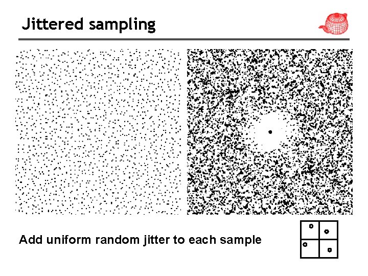
Jittered sampling Add uniform random jitter to each sample

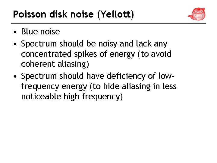
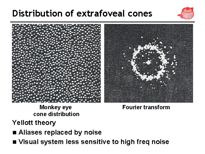
Poisson disk noise (Yellott) • Blue noise • Spectrum should be noisy and lack any concentrated spikes of energy (to avoid coherent aliasing) • Spectrum should have deficiency of lowfrequency energy (to hide aliasing in less noticeable high frequency)

Distribution of extrafoveal cones Monkey eye cone distribution Fourier transform Yellott theory n Aliases replaced by noise n Visual system less sensitive to high freq noise

Example

Aliasing frequency domain function (a) function (b) alias=false frequency

Stochastic sampling

Stochastic sampling function (a) function (b) Replace structure alias by structureless (high-freq) noise

Antialiasing (adaptive sampling) • Take more samples only when necessary. However, in practice, it is hard to know where we need supersampling. Some heuristics could be used. • It only makes a less aliased image, but may not be more efficient than simple supersampling particular for complex scenes.

Application to ray tracing • Sources of aliasing: object boundary, small objects, textures and materials • Good news: we can do sampling easily • Bad news: we can’t do prefiltering (because we do not have the whole function) • Key insight: we can never remove all aliasing, so we develop techniques to mitigate its impact on the quality of the final image.

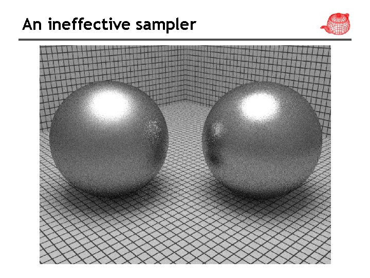
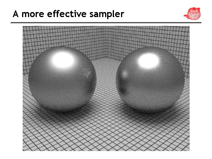
pbrt sampling interface • Creating good sample patterns can substantially improve a ray tracer’s efficiency, allowing it to create a high-quality image with fewer rays. • Because evaluating radiance is costly, it pays to spend time on generating better sampling. • core/sampling. *, samplers/* • random. cpp, stratified. cpp, bestcandidate. cpp, lowdiscrepancy. cpp,

An ineffective sampler

A more effective sampler

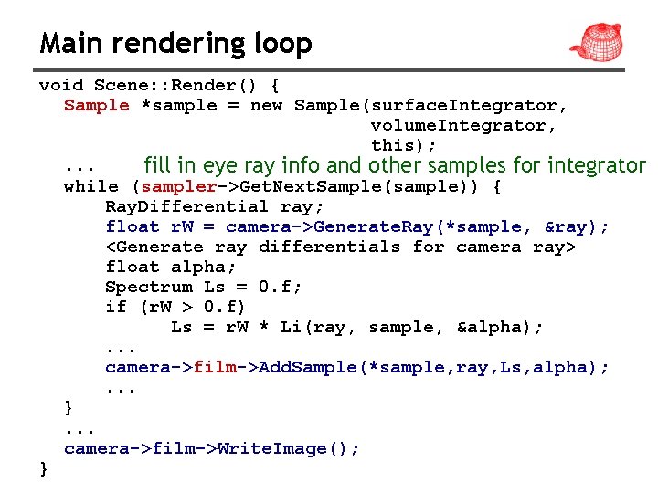
Main rendering loop void Scene: : Render() { Sample *sample = new Sample(surface. Integrator, volume. Integrator, this); . . . fill in eye ray info and other samples for integrator while (sampler->Get. Next. Sample(sample)) { Ray. Differential ray; float r. W = camera->Generate. Ray(*sample, &ray); <Generate ray differentials for camera ray> float alpha; Spectrum Ls = 0. f; if (r. W > 0. f) Ls = r. W * Li(ray, sample, &alpha); . . . camera->film->Add. Sample(*sample, ray, Ls, alpha); . . . }. . . camera->film->Write. Image(); }

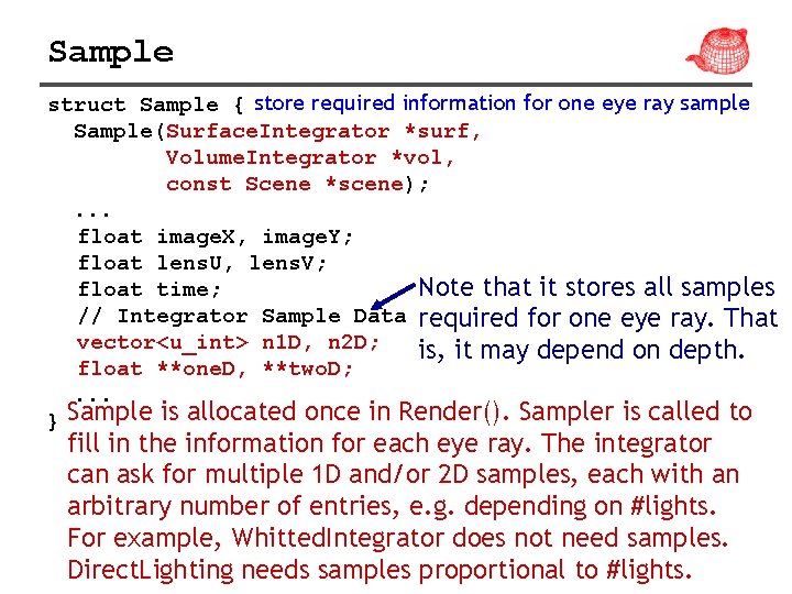
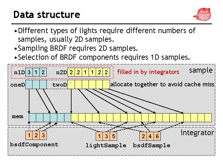
Sample struct Sample { store required information for one eye ray sample Sample(Surface. Integrator *surf, Volume. Integrator *vol, const Scene *scene); . . . float image. X, image. Y; float lens. U, lens. V; Note that it stores all samples float time; // Integrator Sample Data required for one eye ray. That vector<u_int> n 1 D, n 2 D; is, it may depend on depth. float **one. D, **two. D; . . . } Sample is allocated once in Render(). Sampler is called to fill in the information for each eye ray. The integrator can ask for multiple 1 D and/or 2 D samples, each with an arbitrary number of entries, e. g. depending on #lights. For example, Whitted. Integrator does not need samples. Direct. Lighting needs samples proportional to #lights.

Data structure • Different types of lights require different numbers of samples, usually 2 D samples. • Sampling BRDF requires 2 D samples. • Selection of BRDF components requires 1 D samples. n 1 D 3 1 2 one. D filled in by integrators n 2 D 2 2 1 1 2 2 two. D sample allocate together to avoid cache miss mem 1 2 3 bsdf. Component 1 3 5 2 4 6 light. Sample bsdf. Sample integrator

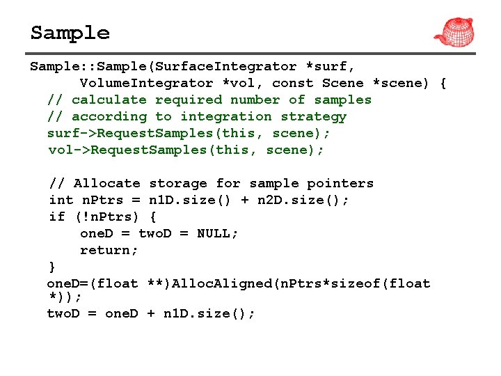
Sample: : Sample(Surface. Integrator *surf, Volume. Integrator *vol, const Scene *scene) { // calculate required number of samples // according to integration strategy surf->Request. Samples(this, scene); vol->Request. Samples(this, scene); // Allocate storage for sample pointers int n. Ptrs = n 1 D. size() + n 2 D. size(); if (!n. Ptrs) { one. D = two. D = NULL; return; } one. D=(float **)Alloc. Aligned(n. Ptrs*sizeof(float *)); two. D = one. D + n 1 D. size();

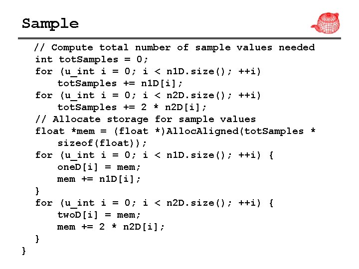
Sample // Compute total number of sample values needed int tot. Samples = 0; for (u_int i = 0; i < n 1 D. size(); ++i) tot. Samples += n 1 D[i]; for (u_int i = 0; i < n 2 D. size(); ++i) tot. Samples += 2 * n 2 D[i]; // Allocate storage for sample values float *mem = (float *)Alloc. Aligned(tot. Samples * sizeof(float)); for (u_int i = 0; i < n 1 D. size(); ++i) { one. D[i] = mem; mem += n 1 D[i]; } for (u_int i = 0; i < n 2 D. size(); ++i) { two. D[i] = mem; mem += 2 * n 2 D[i]; } }

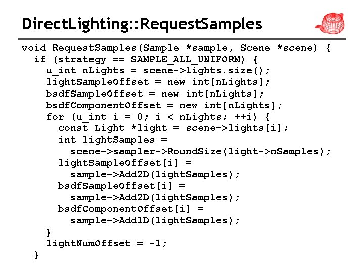
Direct. Lighting: : Request. Samples void Request. Samples(Sample *sample, Scene *scene) { if (strategy == SAMPLE_ALL_UNIFORM) { u_int n. Lights = scene->lights. size(); light. Sample. Offset = new int[n. Lights]; bsdf. Component. Offset = new int[n. Lights]; for (u_int i = 0; i < n. Lights; ++i) { const Light *light = scene->lights[i]; int light. Samples = scene->sampler->Round. Size(light->n. Samples); light. Sample. Offset[i] = sample->Add 2 D(light. Samples); bsdf. Component. Offset[i] = sample->Add 1 D(light. Samples); } light. Num. Offset = -1; }

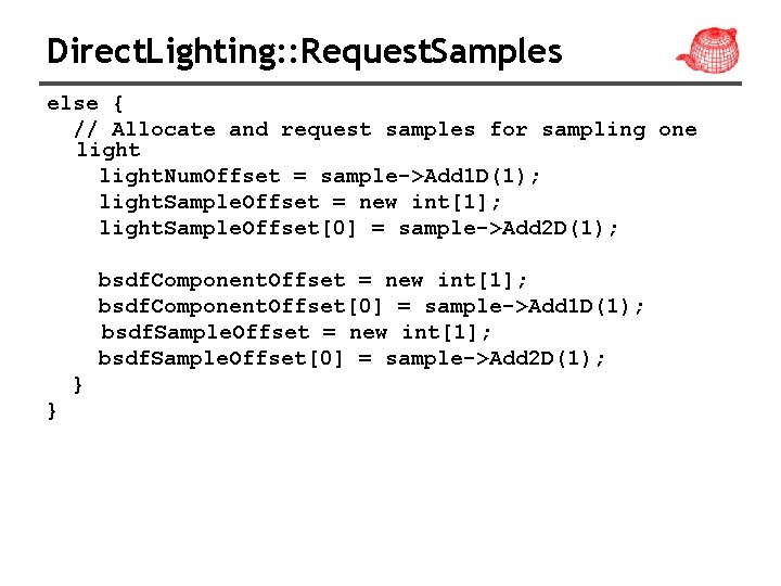
Direct. Lighting: : Request. Samples else { // Allocate and request samples for sampling one light. Num. Offset = sample->Add 1 D(1); light. Sample. Offset = new int[1]; light. Sample. Offset[0] = sample->Add 2 D(1); bsdf. Component. Offset = new int[1]; bsdf. Component. Offset[0] = sample->Add 1 D(1); bsdf. Sample. Offset = new int[1]; bsdf. Sample. Offset[0] = sample->Add 2 D(1); } }

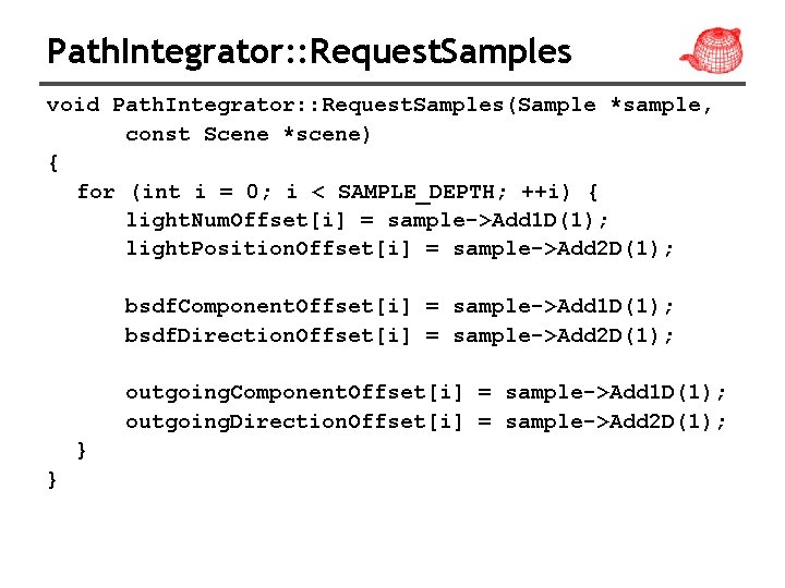
Path. Integrator: : Request. Samples void Path. Integrator: : Request. Samples(Sample *sample, const Scene *scene) { for (int i = 0; i < SAMPLE_DEPTH; ++i) { light. Num. Offset[i] = sample->Add 1 D(1); light. Position. Offset[i] = sample->Add 2 D(1); bsdf. Component. Offset[i] = sample->Add 1 D(1); bsdf. Direction. Offset[i] = sample->Add 2 D(1); outgoing. Component. Offset[i] = sample->Add 1 D(1); outgoing. Direction. Offset[i] = sample->Add 2 D(1); } }

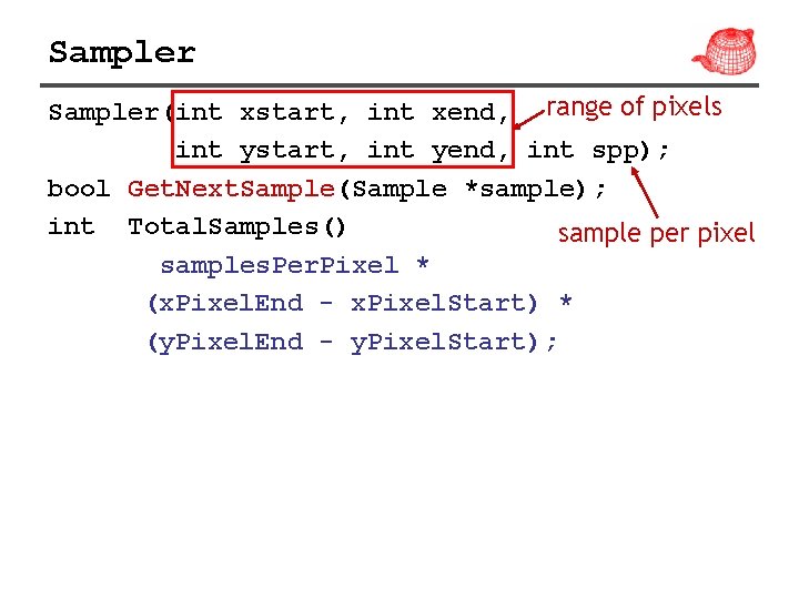
Sampler(int xstart, int xend, range of pixels int ystart, int yend, int spp); bool Get. Next. Sample(Sample *sample); int Total. Samples() sample per pixel samples. Per. Pixel * (x. Pixel. End - x. Pixel. Start) * (y. Pixel. End - y. Pixel. Start);

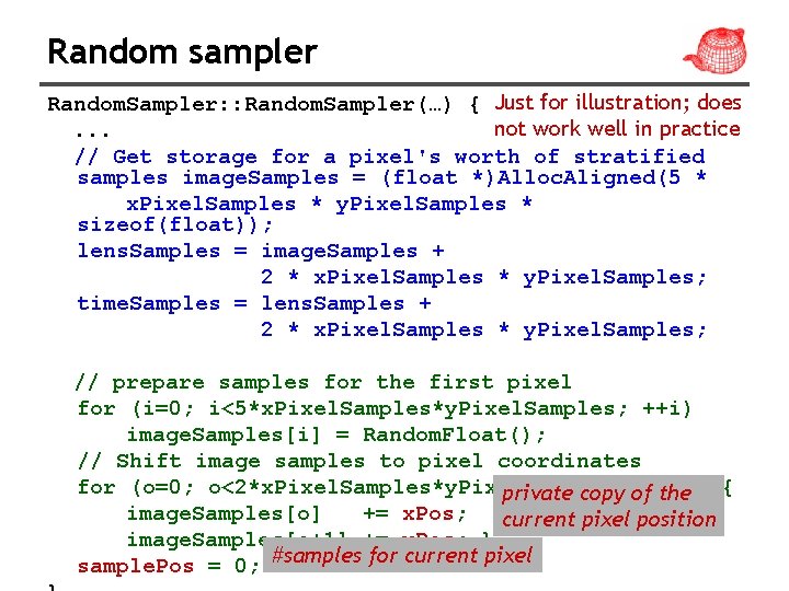
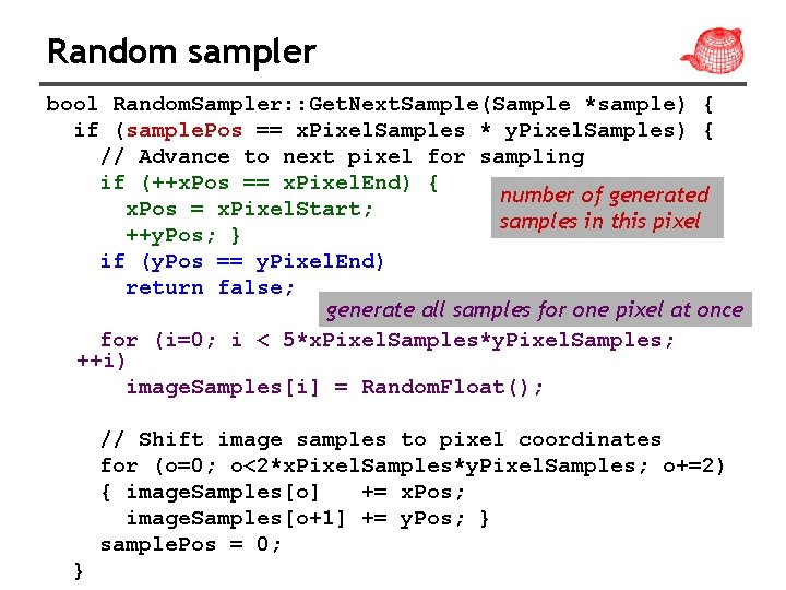
Random sampler Random. Sampler: : Random. Sampler(…) { Just for illustration; does not work well in practice. . . // Get storage for a pixel's worth of stratified samples image. Samples = (float *)Alloc. Aligned(5 * x. Pixel. Samples * y. Pixel. Samples * sizeof(float)); lens. Samples = image. Samples + 2 * x. Pixel. Samples * y. Pixel. Samples; time. Samples = lens. Samples + 2 * x. Pixel. Samples * y. Pixel. Samples; // prepare samples for the first pixel for (i=0; i<5*x. Pixel. Samples*y. Pixel. Samples; ++i) image. Samples[i] = Random. Float(); // Shift image samples to pixel coordinates for (o=0; o<2*x. Pixel. Samples*y. Pixel. Samples; private copy ofo+=2) the { image. Samples[o] += x. Pos; current pixel position image. Samples[o+1] += y. Pos; } sample. Pos = 0; #samples for current pixel

Random sampler bool Random. Sampler: : Get. Next. Sample(Sample *sample) { if (sample. Pos == x. Pixel. Samples * y. Pixel. Samples) { // Advance to next pixel for sampling if (++x. Pos == x. Pixel. End) { number of generated x. Pos = x. Pixel. Start; samples in this pixel ++y. Pos; } if (y. Pos == y. Pixel. End) return false; generate all samples for one pixel at once for (i=0; i < 5*x. Pixel. Samples*y. Pixel. Samples; ++i) image. Samples[i] = Random. Float(); // Shift image samples to pixel coordinates for (o=0; o<2*x. Pixel. Samples*y. Pixel. Samples; o+=2) { image. Samples[o] += x. Pos; image. Samples[o+1] += y. Pos; } sample. Pos = 0; }

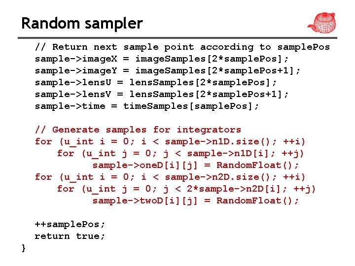
Random sampler // Return next sample point according to sample. Pos sample->image. X = image. Samples[2*sample. Pos]; sample->image. Y = image. Samples[2*sample. Pos+1]; sample->lens. U = lens. Samples[2*sample. Pos]; sample->lens. V = lens. Samples[2*sample. Pos+1]; sample->time = time. Samples[sample. Pos]; // Generate samples for integrators for (u_int i = 0; i < sample->n 1 D. size(); ++i) for (u_int j = 0; j < sample->n 1 D[i]; ++j) sample->one. D[i][j] = Random. Float(); for (u_int i = 0; i < sample->n 2 D. size(); ++i) for (u_int j = 0; j < 2*sample->n 2 D[i]; ++j) sample->two. D[i][j] = Random. Float(); ++sample. Pos; return true; }

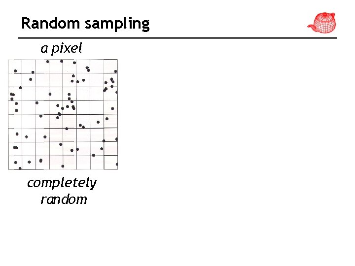
Random sampling a pixel completely random

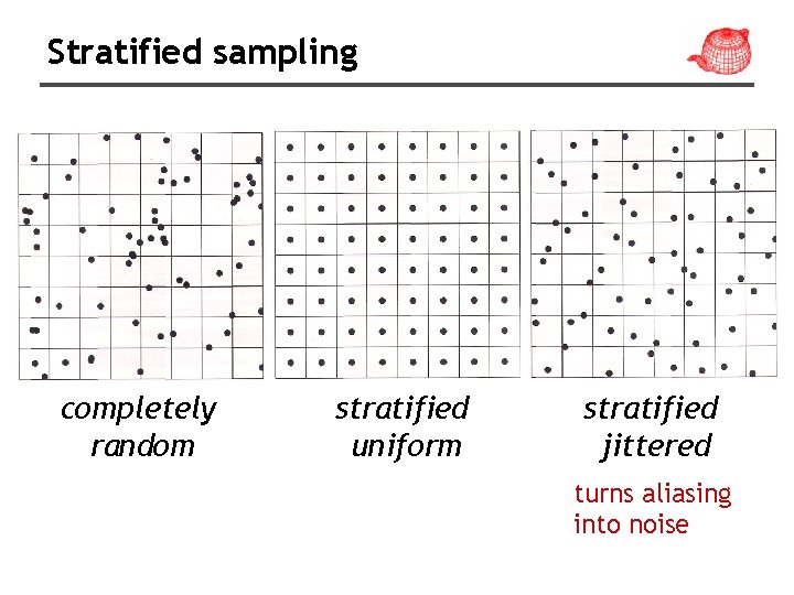
Stratified sampling • Subdivide the sampling domain into nonoverlapping regions (strata) and take a single sample from each one so that it is less likely to miss important features.

Stratified sampling completely random stratified uniform stratified jittered turns aliasing into noise

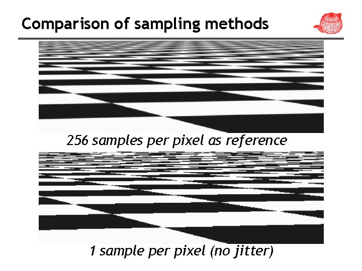
Comparison of sampling methods 256 samples per pixel as reference 1 sample per pixel (no jitter)

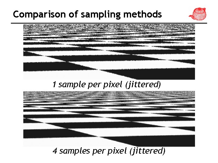
Comparison of sampling methods 1 sample per pixel (jittered) 4 samples per pixel (jittered)

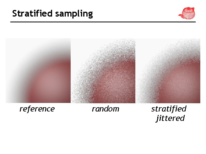
Stratified sampling reference random stratified jittered

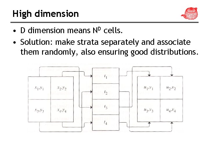
High dimension • D dimension means ND cells. • Solution: make strata separately and associate them randomly, also ensuring good distributions.

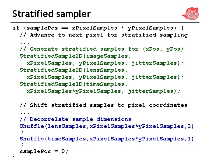
Stratified sampler if (sample. Pos == x. Pixel. Samples * y. Pixel. Samples) { // Advance to next pixel for stratified sampling. . . // Generate stratified samples for (x. Pos, y. Pos) Stratified. Sample 2 D(image. Samples, x. Pixel. Samples, y. Pixel. Samples, jitter. Samples); Stratified. Sample 2 D(lens. Samples, x. Pixel. Samples, y. Pixel. Samples, jitter. Samples); Stratified. Sample 1 D(time. Samples, x. Pixel. Samples*y. Pixel. Samples, jitter. Samples); // Shift stratified samples to pixel coordinates. . . // Decorrelate sample dimensions Shuffle(lens. Samples, x. Pixel. Samples*y. Pixel. Samples, 2) ; Shuffle(time. Samples, x. Pixel. Samples*y. Pixel. Samples, 1) ; sample. Pos = 0;

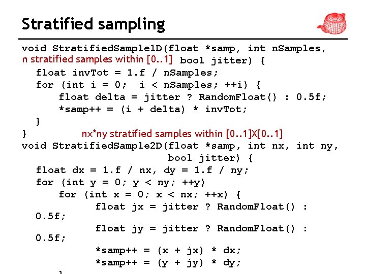
Stratified sampling void Stratified. Sample 1 D(float *samp, int n. Samples, n stratified samples within [0. . 1] bool jitter) { float inv. Tot = 1. f / n. Samples; for (int i = 0; i < n. Samples; ++i) { float delta = jitter ? Random. Float() : 0. 5 f; *samp++ = (i + delta) * inv. Tot; } } nx*ny stratified samples within [0. . 1]X[0. . 1] void Stratified. Sample 2 D(float *samp, int nx, int ny, bool jitter) { float dx = 1. f / nx, dy = 1. f / ny; for (int y = 0; y < ny; ++y) for (int x = 0; x < nx; ++x) { float jx = jitter ? Random. Float() : 0. 5 f; float jy = jitter ? Random. Float() : 0. 5 f; *samp++ = (x + jx) * dx; *samp++ = (y + jy) * dy;

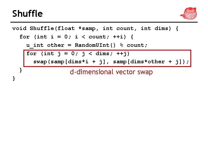
Shuffle void Shuffle(float *samp, int count, int dims) { for (int i = 0; i < count; ++i) { u_int other = Random. UInt() % count; for (int j = 0; j < dims; ++j) swap(samp[dims*i + j], samp[dims*other + j]); } d-dimensional vector swap }

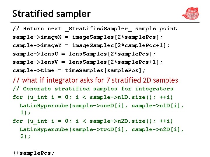
Stratified sampler // Return next _Stratified. Sampler_ sample point sample->image. X = image. Samples[2*sample. Pos]; sample->image. Y = image. Samples[2*sample. Pos+1]; sample->lens. U = lens. Samples[2*sample. Pos]; sample->lens. V = lens. Samples[2*sample. Pos+1]; sample->time = time. Samples[sample. Pos]; // what if integrator asks for 7 stratified 2 D samples // Generate stratified samples for integrators for (u_int i = 0; i < sample->n 1 D. size(); ++i) Latin. Hypercube(sample->one. D[i], sample->n 1 D[i], 1); for (u_int i = 0; i < sample->n 2 D. size(); ++i) Latin. Hypercube(sample->two. D[i], sample->n 2 D[i], 2); ++sample. Pos;

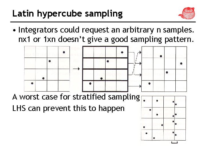
Latin hypercube sampling • Integrators could request an arbitrary n samples. nx 1 or 1 xn doesn’t give a good sampling pattern. A worst case for stratified sampling LHS can prevent this to happen

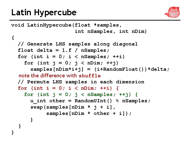
Latin Hypercube void Latin. Hypercube(float *samples, int n. Samples, int n. Dim) { // Generate LHS samples along diagonal float delta = 1. f / n. Samples; for (int i = 0; i < n. Samples; ++i) for (int j = 0; j < n. Dim; ++j) samples[n. Dim*i+j] = (i+Random. Float())*delta; note the difference with shuffle // Permute LHS samples in each dimension for (int i = 0; i < n. Dim; ++i) { for (int j = 0; j < n. Samples; ++j) { u_int other = Random. UInt() % n. Samples; swap(samples[n. Dim * j + i], samples[n. Dim * other + i]); } } }

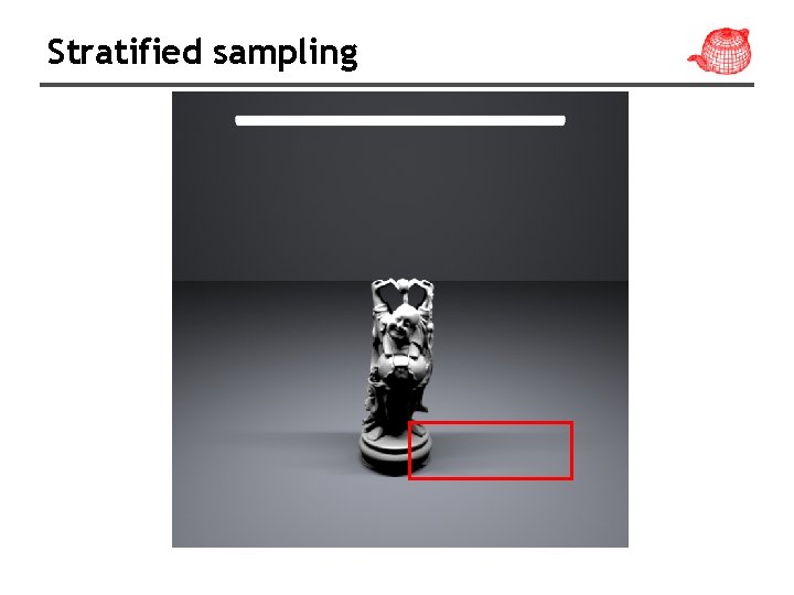
Stratified sampling

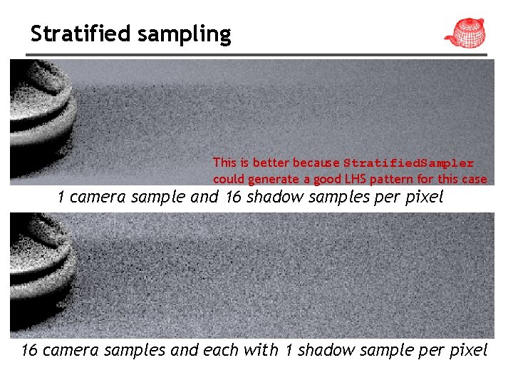
Stratified sampling This is better because Stratified. Sampler could generate a good LHS pattern for this case 1 camera sample and 16 shadow samples per pixel 16 camera samples and each with 1 shadow sample per pixel

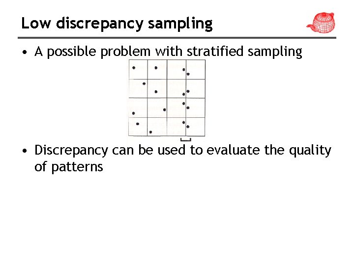
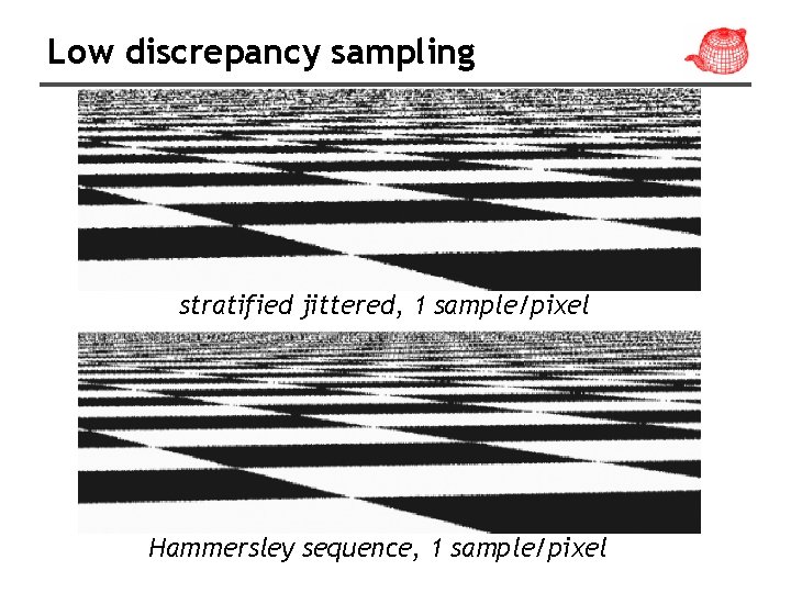
Low discrepancy sampling • A possible problem with stratified sampling • Discrepancy can be used to evaluate the quality of patterns

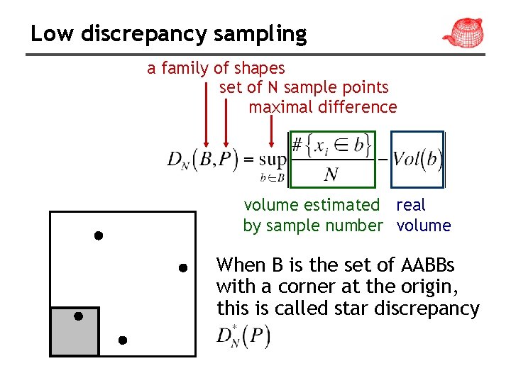
Low discrepancy sampling a family of shapes set of N sample points maximal difference volume estimated real by sample number volume When B is the set of AABBs with a corner at the origin, this is called star discrepancy

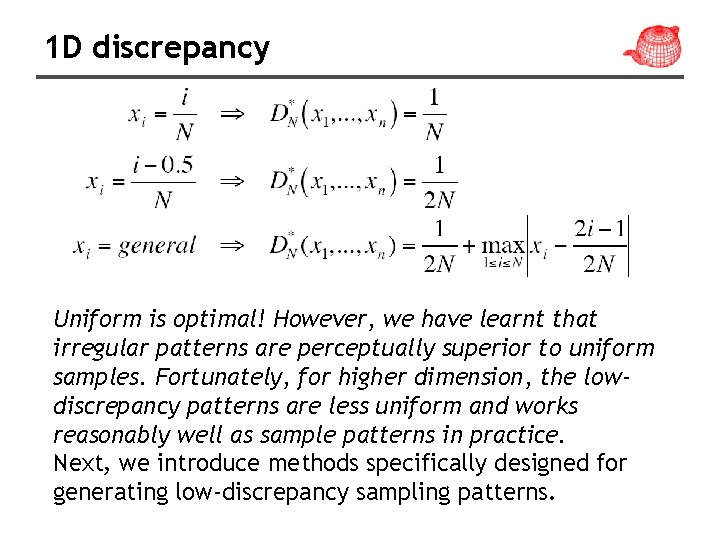
1 D discrepancy Uniform is optimal! However, we have learnt that irregular patterns are perceptually superior to uniform samples. Fortunately, for higher dimension, the lowdiscrepancy patterns are less uniform and works reasonably well as sample patterns in practice. Next, we introduce methods specifically designed for generating low-discrepancy sampling patterns.

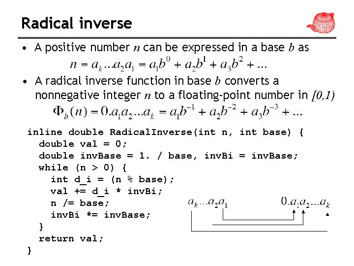
Radical inverse • A positive number n can be expressed in a base b as • A radical inverse function in base b converts a nonnegative integer n to a floating-point number in [0, 1) inline double Radical. Inverse(int n, int base) { double val = 0; double inv. Base = 1. / base, inv. Bi = inv. Base; while (n > 0) { int d_i = (n % base); val += d_i * inv. Bi; n /= base; inv. Bi *= inv. Base; } return val; }

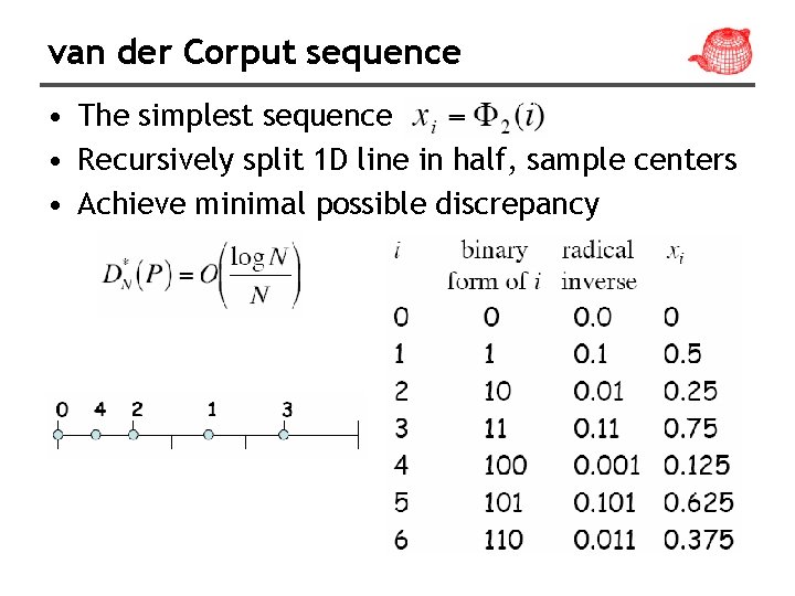
van der Corput sequence • The simplest sequence • Recursively split 1 D line in half, sample centers • Achieve minimal possible discrepancy

High-dimensional sequence • Two well-known low-discrepancy sequences – Halton – Hammersley

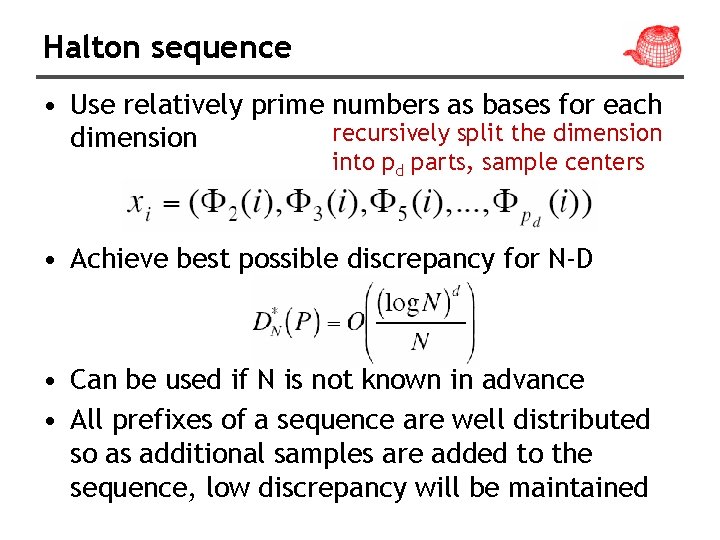
Halton sequence • Use relatively prime numbers as bases for each recursively split the dimension into pd parts, sample centers • Achieve best possible discrepancy for N-D • Can be used if N is not known in advance • All prefixes of a sequence are well distributed so as additional samples are added to the sequence, low discrepancy will be maintained

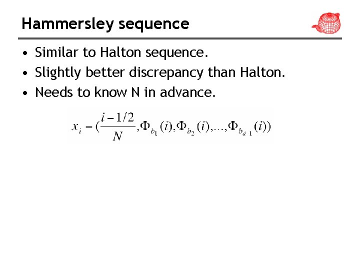
Hammersley sequence • Similar to Halton sequence. • Slightly better discrepancy than Halton. • Needs to know N in advance.

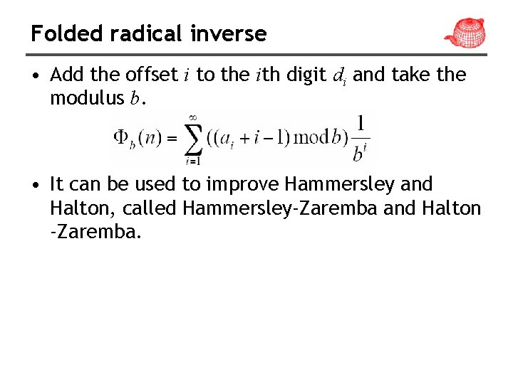
Folded radical inverse • Add the offset i to the ith digit di and take the modulus b. • It can be used to improve Hammersley and Halton, called Hammersley-Zaremba and Halton -Zaremba.

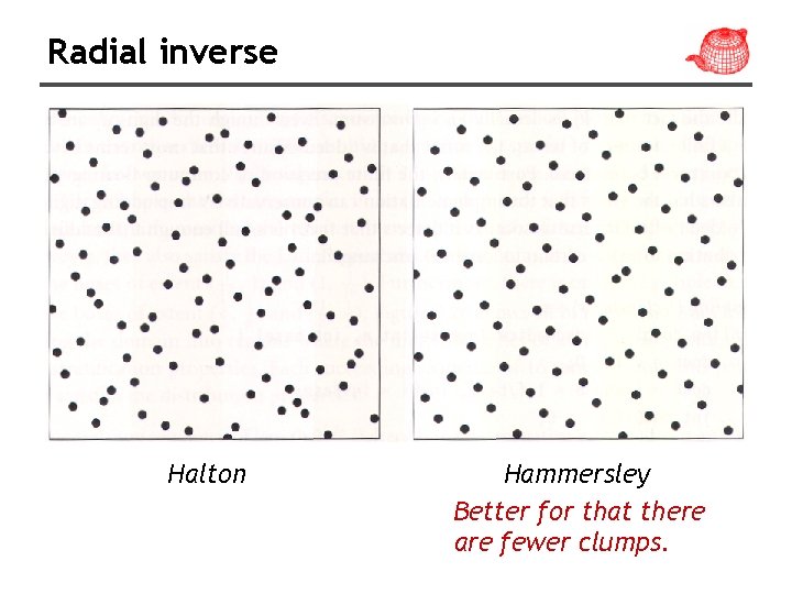
Radial inverse Halton Hammersley Better for that there are fewer clumps.

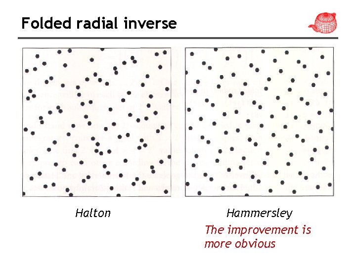
Folded radial inverse Halton Hammersley The improvement is more obvious

Low discrepancy sampling stratified jittered, 1 sample/pixel Hammersley sequence, 1 sample/pixel

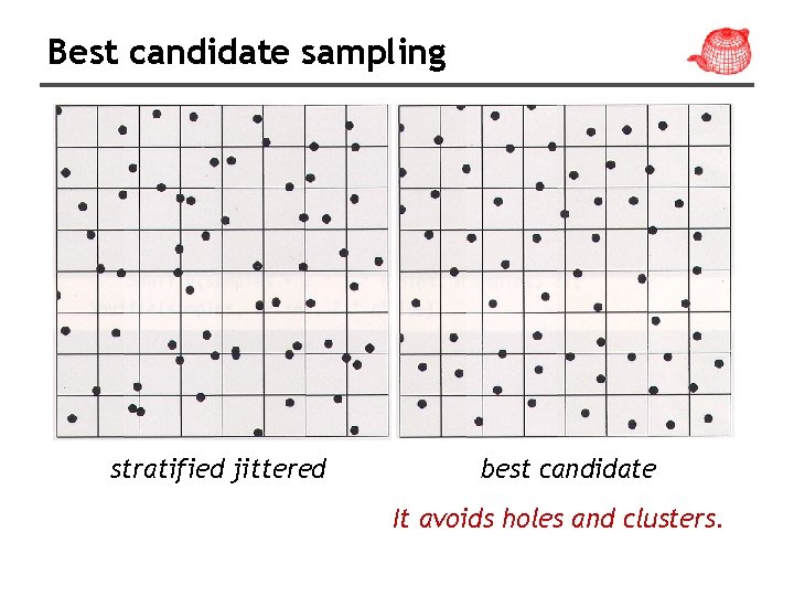
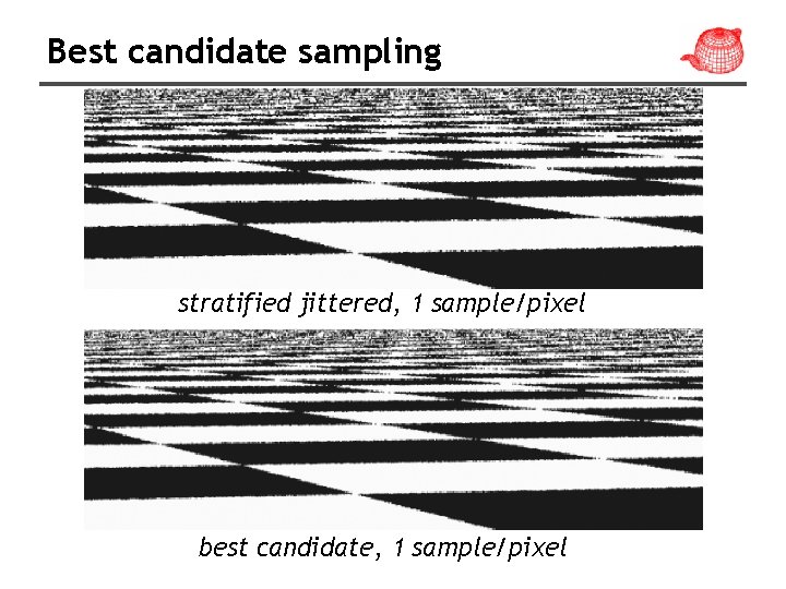
Best candidate sampling • Stratified sampling doesn’t guarantee good sampling across pixels. • Poisson disk pattern addresses this issue. The Poisson disk pattern is a group of points with no two of them closer to each other than some specified distance. • It can be generated by dart throwing. It is timeconsuming. • Best-candidate algorithm by Dan Mitchell. It randomly generates many candidates but only inserts the one farthest to all previous samples.

Best candidate sampling stratified jittered best candidate It avoids holes and clusters.

Best candidate sampling • Because of it is costly to generate best candidate pattern, pbrt computes a “tilable pattern” offline (by treating the square as a rolled torus). • tools/samplepat. cpp→sampler/sampledata. cpp

Best candidate sampling stratified jittered, 1 sample/pixel best candidate, 1 sample/pixel

Best candidate sampling stratified jittered, 4 sample/pixel best candidate, 4 sample/pixel

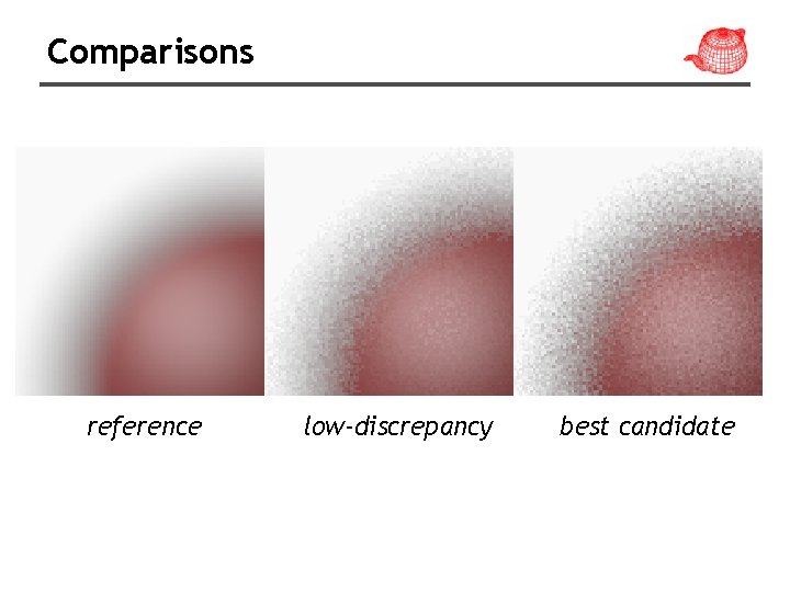
Comparisons reference low-discrepancy best candidate

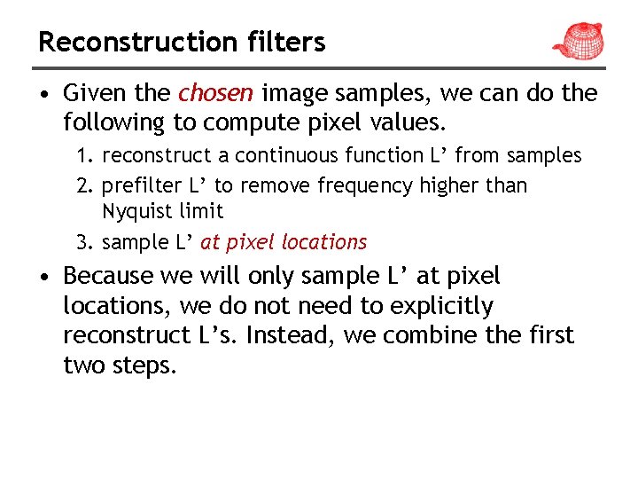
Reconstruction filters • Given the chosen image samples, we can do the following to compute pixel values. 1. reconstruct a continuous function L’ from samples 2. prefilter L’ to remove frequency higher than Nyquist limit 3. sample L’ at pixel locations • Because we will only sample L’ at pixel locations, we do not need to explicitly reconstruct L’s. Instead, we combine the first two steps.

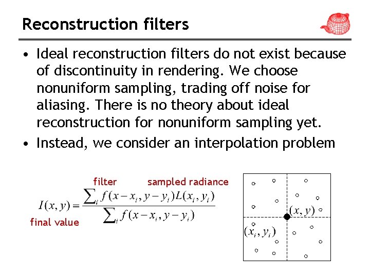
Reconstruction filters • Ideal reconstruction filters do not exist because of discontinuity in rendering. We choose nonuniform sampling, trading off noise for aliasing. There is no theory about ideal reconstruction for nonuniform sampling yet. • Instead, we consider an interpolation problem filter final value sampled radiance

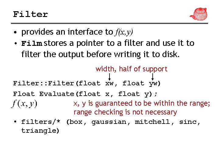
Filter • provides an interface to f(x, y) • Film stores a pointer to a filter and use it to filter the output before writing it to disk. width, half of support Filter: : Filter(float xw, float yw) Float Evaluate(float x, float y); x, y is guaranteed to be within the range; range checking is not necessary • filters/* (box, gaussian, mitchell, sinc, triangle)

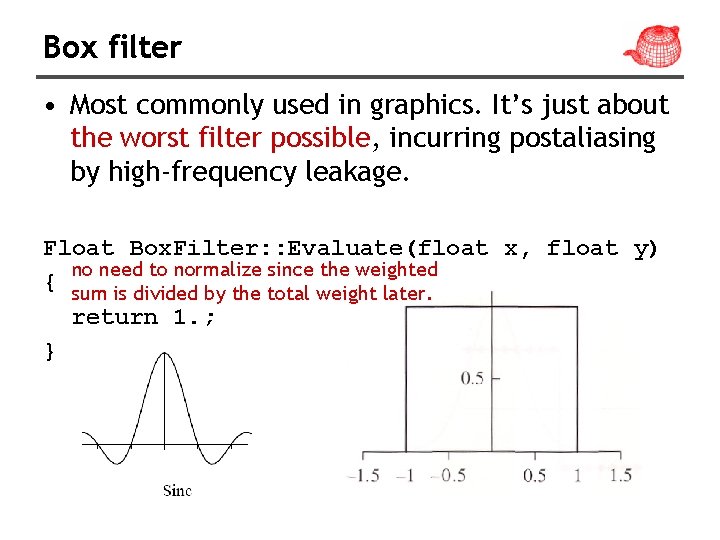
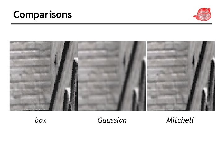
Box filter • Most commonly used in graphics. It’s just about the worst filter possible, incurring postaliasing by high-frequency leakage. Float Box. Filter: : Evaluate(float x, float y) no need to normalize since the weighted { sum is divided by the total weight later. return 1. ; }

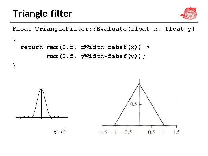
Triangle filter Float Triangle. Filter: : Evaluate(float x, float y) { return max(0. f, x. Width-fabsf(x)) * max(0. f, y. Width-fabsf(y)); }

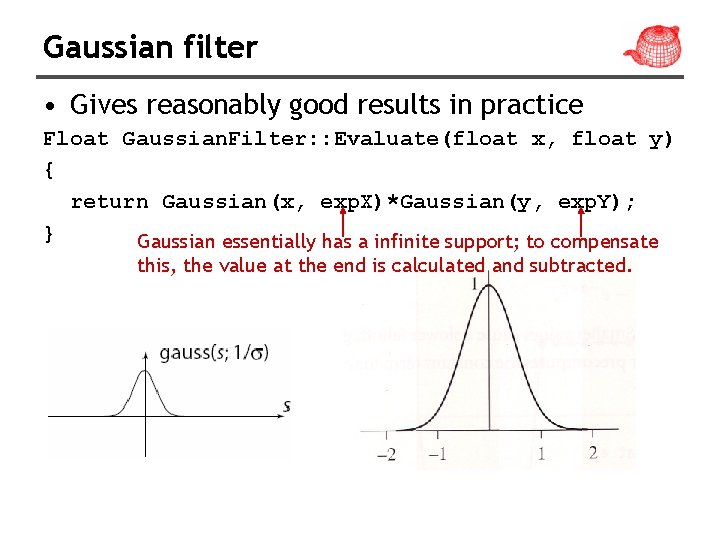
Gaussian filter • Gives reasonably good results in practice Float Gaussian. Filter: : Evaluate(float x, float y) { return Gaussian(x, exp. X)*Gaussian(y, exp. Y); } Gaussian essentially has a infinite support; to compensate this, the value at the end is calculated and subtracted.

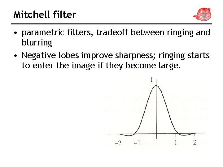
Mitchell filter • parametric filters, tradeoff between ringing and blurring • Negative lobes improve sharpness; ringing starts to enter the image if they become large.

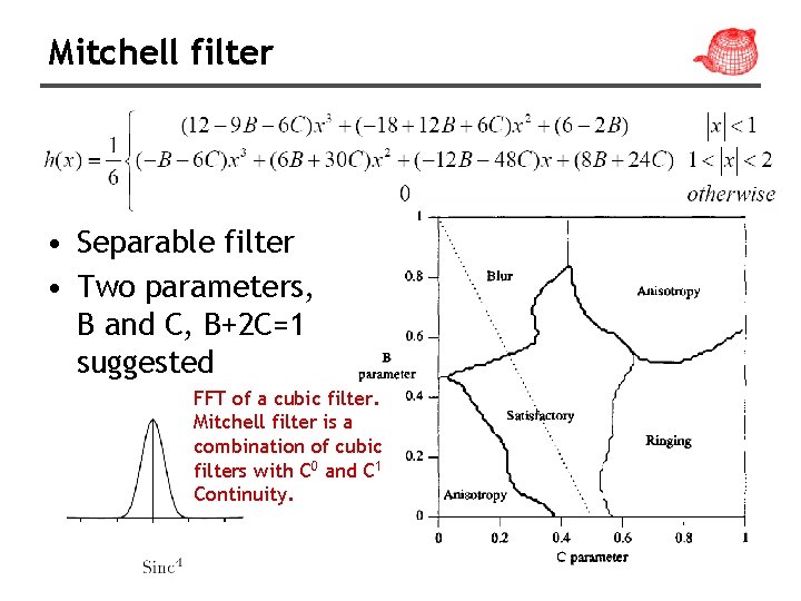
Mitchell filter • Separable filter • Two parameters, B and C, B+2 C=1 suggested FFT of a cubic filter. Mitchell filter is a combination of cubic filters with C 0 and C 1 Continuity.

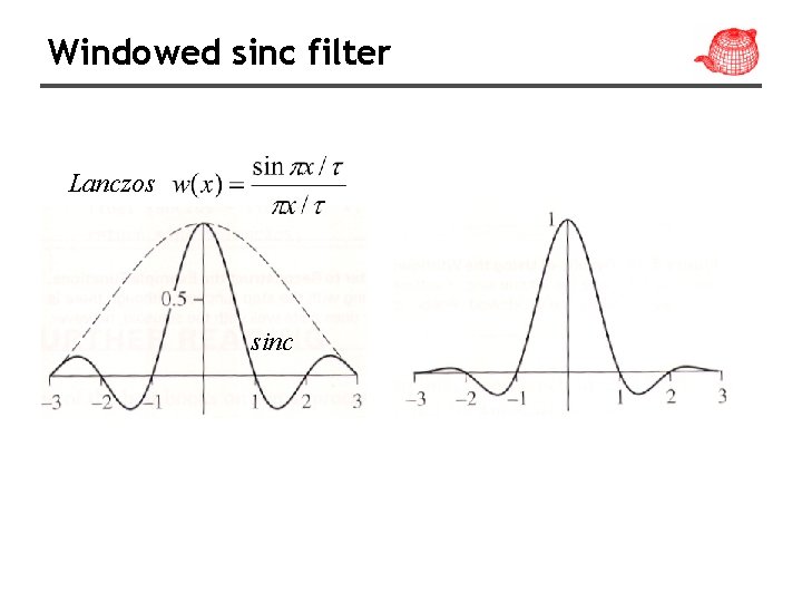
Windowed sinc filter Lanczos sinc

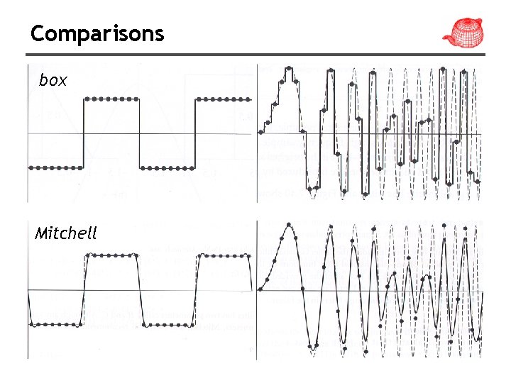
Comparisons box Mitchell

Comparisons windowed sinc Mitchell

Comparisons box Gaussian Mitchell

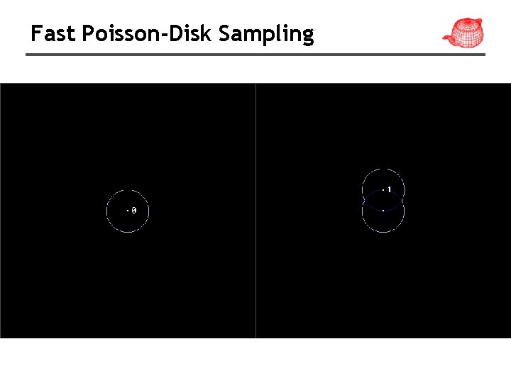
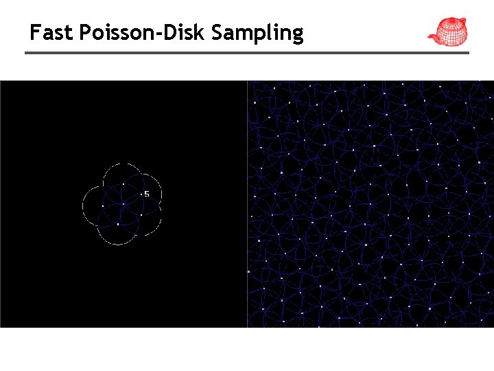
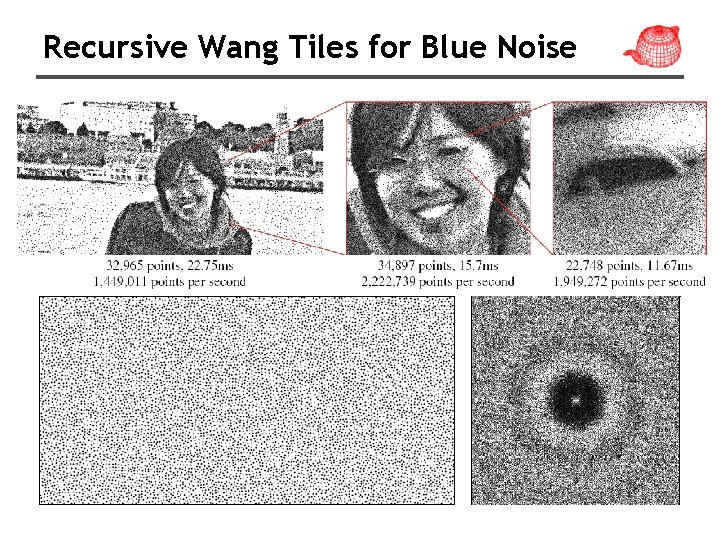
Recent progresses on Poisson sampling • On-the-fly computing – Scalloped regions [SIGGRAPH 2006] • Tile-based – Recursive Wang tile [SIGGRAPH 2006] • Parallel – Li-Yi Wei [SIGGRAPH 2008] • Show three videos for them

Fast Poisson-Disk Sampling

Fast Poisson-Disk Sampling

Recursive Wang Tiles for Blue Noise