Effect Sizes ES for MetaAnalyses ES d reta

Effect Sizes (ES) for Meta-Analyses • ES – d, r/eta & OR • computing ESs • estimating ESs • ESs to beware! • interpreting ES • ES transformations • ES adustments • outlier identification

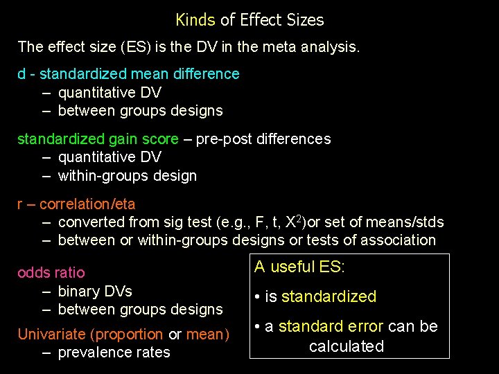
Kinds of Effect Sizes The effect size (ES) is the DV in the meta analysis. d - standardized mean difference – quantitative DV – between groups designs standardized gain score – pre-post differences – quantitative DV – within-groups design r – correlation/eta – converted from sig test (e. g. , F, t, X 2)or set of means/stds – between or within-groups designs or tests of association odds ratio – binary DVs – between groups designs Univariate (proportion or mean) – prevalence rates A useful ES: • is standardized • a standard error can be calculated

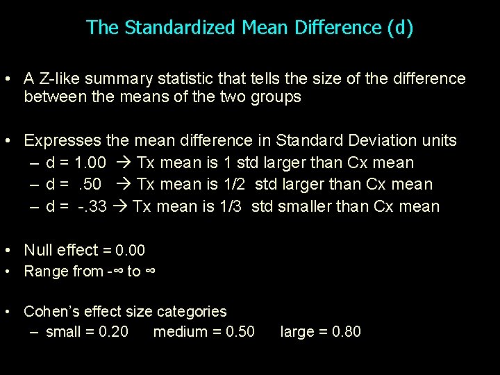
The Standardized Mean Difference (d) • A Z-like summary statistic that tells the size of the difference between the means of the two groups • Expresses the mean difference in Standard Deviation units – d = 1. 00 Tx mean is 1 std larger than Cx mean – d =. 50 Tx mean is 1/2 std larger than Cx mean – d = -. 33 Tx mean is 1/3 std smaller than Cx mean • Null effect = 0. 00 • Range from -∞ to ∞ • Cohen’s effect size categories – small = 0. 20 medium = 0. 50 large = 0. 80

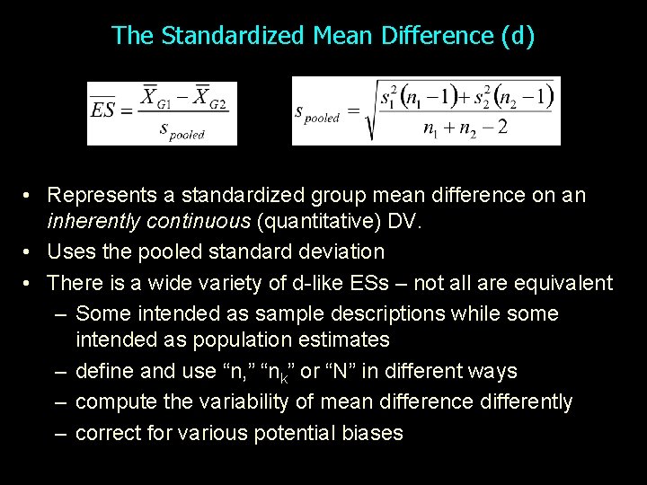
The Standardized Mean Difference (d) • Represents a standardized group mean difference on an inherently continuous (quantitative) DV. • Uses the pooled standard deviation • There is a wide variety of d-like ESs – not all are equivalent – Some intended as sample descriptions while some intended as population estimates – define and use “n, ” “nk” or “N” in different ways – compute the variability of mean difference differently – correct for various potential biases

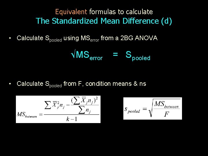
Equivalent formulas to calculate The Standardized Mean Difference (d) • Calculate Spooled using MSerror from a 2 BG ANOVA √MSerror = Spooled • Calculate Spooled from F, condition means & ns

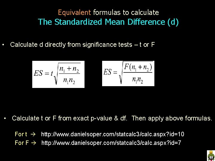
Equivalent formulas to calculate The Standardized Mean Difference (d) • Calculate d directly from significance tests – t or F • Calculate t or F from exact p-value & df. Then apply above formulas. For t http: //www. danielsoper. com/statcalc 3/calc. aspx? id=10 For F http: //www. danielsoper. com/statcalc 3/calc. aspx? id=7

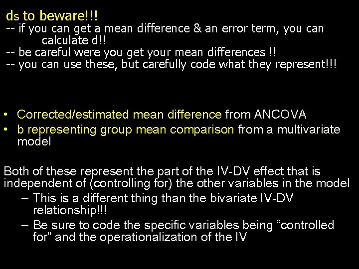
ds to beware!!! -- if you can get a mean difference & an error term, you can calculate d!! -- be careful were you get your mean differences !! -- you can use these, but carefully code what they represent!!! • Corrected/estimated mean difference from ANCOVA • b representing group mean comparison from a multivariate model Both of these represent the part of the IV-DV effect that is independent of (controlling for) the other variables in the model – This is a different thing than the bivariate IV-DV relationship!!! – Be sure to code the specific variables being “controlled for” and the operationalization of the IV

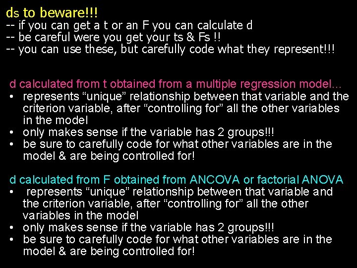
ds to beware!!! -- if you can get a t or an F you can calculate d -- be careful were you get your ts & Fs !! -- you can use these, but carefully code what they represent!!! d calculated from t obtained from a multiple regression model… • represents “unique” relationship between that variable and the criterion variable, after “controlling for” all the other variables in the model • only makes sense if the variable has 2 groups!!! • be sure to carefully code for what other variables are in the model & are being controlled for! d calculated from F obtained from ANCOVA or factorial ANOVA • represents “unique” relationship between that variable and the criterion variable, after “controlling for” all the other variables in the model • only makes sense if the variable has 2 groups!!! • be sure to carefully code for what other variables are in the model & are being controlled for!

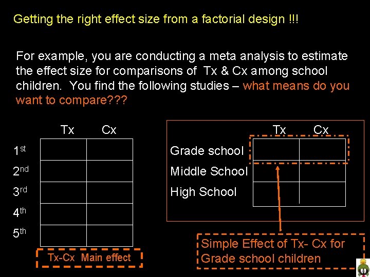
Getting the right effect size from a factorial design !!! For example, you are conducting a meta analysis to estimate the effect size for comparisons of Tx & Cx among school children. You find the following studies – what means do you want to compare? ? ? Tx Cx Tx 1 st Grade school 2 nd Middle School 3 rd High School Cx 4 th 5 th Tx-Cx Main effect Simple Effect of Tx- Cx for Grade school children

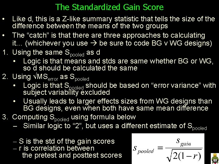
The Standardized Gain Score • Like d, this is a Z-like summary statistic that tells the size of the difference between the means of the two groups • The “catch” is that there are three approaches to calculating it… (whichever you use be sure to code BG v WG designs) 1. Using the same Spooled as d • Logic is that means and stds are same whether BG or WG, so d should be calculated the same 2. Using √MSerror as Spooled • Logic is that Spooled should be based on “error variance” with subject variability excluded • Usually leads to larger effects sizes from WG designs than BG designs, even when both have same mean difference 3. Computing Spooled using formula below – Similar logic to “ 2”, but uses a different estimate of Spooled – S is the std of the gain scores – r is correlation between the pretest and posttest scores

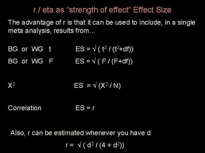
r / eta as “strength of effect” Effect Size The advantage of r is that it can be used to include, in a single meta analysis, results from… BG or WG t ES = √ ( t 2 / (t 2+df)) BG or WG F ES = √ ( F / (F+df)) X 2 ES = √ (X 2 / N) Correlation ES = r Also, r can be estimated whenever you have d r = √ ( d 2 / (4 + d 2))

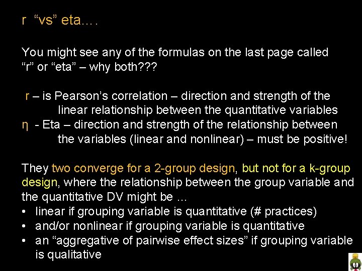
r “vs” eta…. You might see any of the formulas on the last page called “r” or “eta” – why both? ? ? r – is Pearson’s correlation – direction and strength of the linear relationship between the quantitative variables η - Eta – direction and strength of the relationship between the variables (linear and nonlinear) – must be positive! They two converge for a 2 -group design, but not for a k-group design, where the relationship between the group variable and the quantitative DV might be … • linear if grouping variable is quantitative (# practices) • and/or nonlinear if grouping variable is quantitative • an “aggregative of pairwise effect sizes” if grouping variable is qualitative

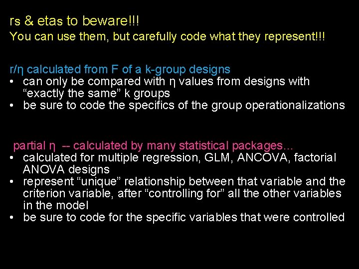
rs & etas to beware!!! You can use them, but carefully code what they represent!!! r/η calculated from F of a k-group designs • can only be compared with η values from designs with “exactly the same” k groups • be sure to code the specifics of the group operationalizations partial η -- calculated by many statistical packages… • calculated for multiple regression, GLM, ANCOVA, factorial ANOVA designs • represent “unique” relationship between that variable and the criterion variable, after “controlling for” all the other variables in the model • be sure to code for the specific variables that were controlled

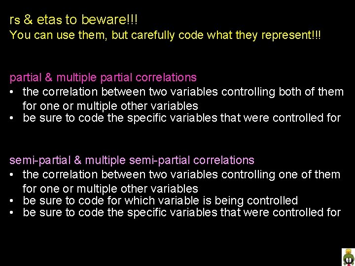
rs & etas to beware!!! You can use them, but carefully code what they represent!!! partial & multiple partial correlations • the correlation between two variables controlling both of them for one or multiple other variables • be sure to code the specific variables that were controlled for semi-partial & multiple semi-partial correlations • the correlation between two variables controlling one of them for one or multiple other variables • be sure to code for which variable is being controlled • be sure to code the specific variables that were controlled for

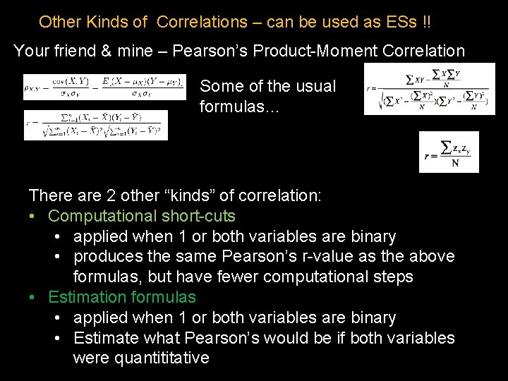
Other Kinds of Correlations – can be used as ESs !! Your friend & mine – Pearson’s Product-Moment Correlation Some of the usual formulas… There are 2 other “kinds” of correlation: • Computational short-cuts • applied when 1 or both variables are binary • produces the same Pearson’s r-value as the above formulas, but have fewer computational steps • Estimation formulas • applied when 1 or both variables are binary • Estimate what Pearson’s would be if both variables were quantititative

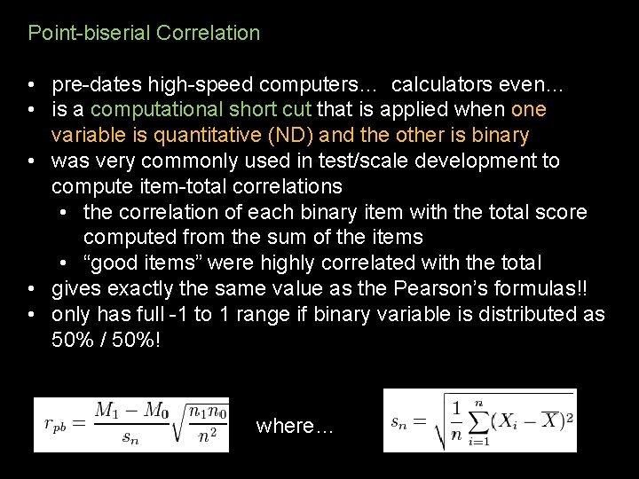
Point-biserial Correlation • pre-dates high-speed computers… calculators even… • is a computational short cut that is applied when one variable is quantitative (ND) and the other is binary • was very commonly used in test/scale development to compute item-total correlations • the correlation of each binary item with the total score computed from the sum of the items • “good items” were highly correlated with the total • gives exactly the same value as the Pearson’s formulas!! • only has full -1 to 1 range if binary variable is distributed as 50% / 50%! where…

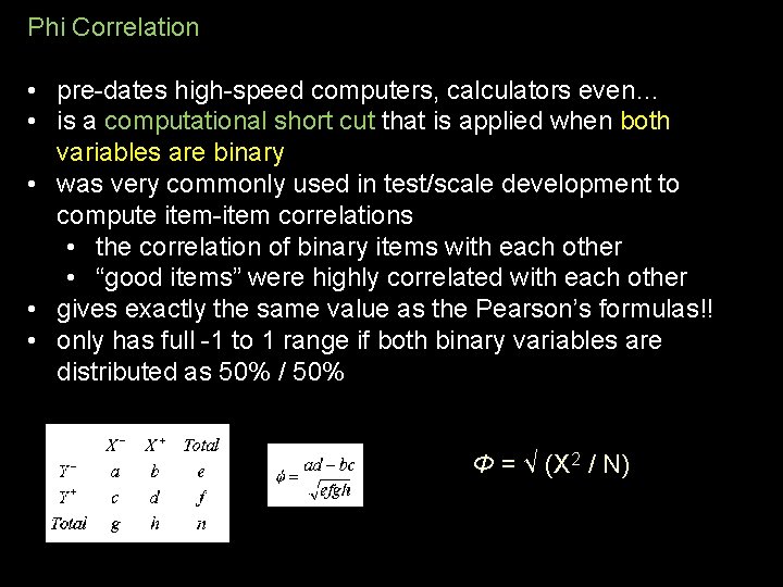
Phi Correlation • pre-dates high-speed computers, calculators even… • is a computational short cut that is applied when both variables are binary • was very commonly used in test/scale development to compute item-item correlations • the correlation of binary items with each other • “good items” were highly correlated with each other • gives exactly the same value as the Pearson’s formulas!! • only has full -1 to 1 range if both binary variables are distributed as 50% / 50% Φ = √ (X 2 / N)

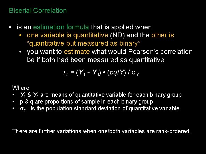
Biserial Correlation • is an estimation formula that is applied when • one variable is quantitative (ND) and the other is “quantitative but measured as binary” • you want to estimate what would Pearson’s correlation be if both had been measured as quantitative rb = (Y 1 - Y 0) • (pq/Y) / σY Where… • Y 1 & Y 0 are means of quantitative variable for each binary group • p & q are proportions of sample in each binary group • σY is the population standard deviation of quantitative variable There are further variations when one/both variables are rank-ordered.

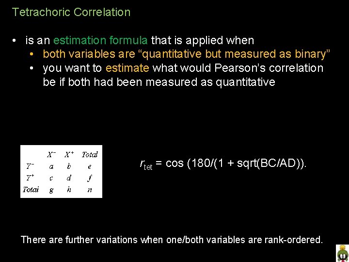
Tetrachoric Correlation • is an estimation formula that is applied when • both variables are “quantitative but measured as binary” • you want to estimate what would Pearson’s correlation be if both had been measured as quantitative rtet = cos (180/(1 + sqrt(BC/AD)). There are further variations when one/both variables are rank-ordered.

The Odds-Ratio • Some meta analysts have pointed out that using the r-type or d-type effect size computed from a 2 x 2 table (binary DV & 2 -group IV can lead to an underestimate of the population effect size, to the extent that the marginal proportions vary from 50/50. • A very workable alternative is to use the Odds-ratio !!! • The odds-ratio is usually described as “the odds of success for Tx members, relative to the odds of success for Cx members. ” – IV = Tx vs. Cx (coded 1 & 0) – DV = Improvement vs. No Improvement (coded 1 & 0) – Odds ratio of 2. 5 means… • Those in the Tx group are 2. 5 times as likely to show improvement as those in the Cx group

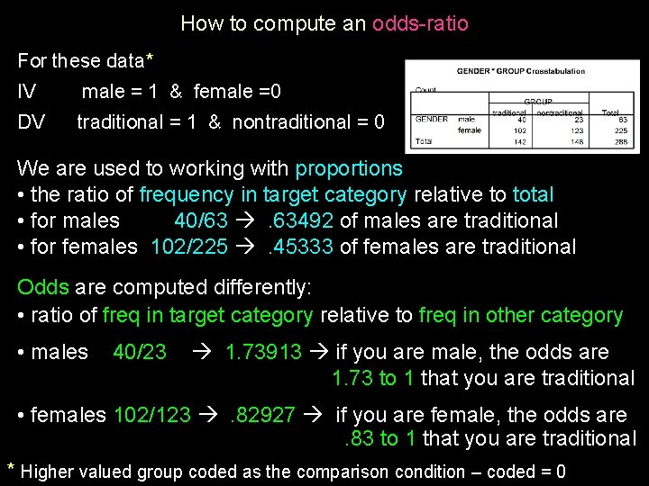
How to compute an odds-ratio For these data* IV male = 1 & female =0 DV traditional = 1 & nontraditional = 0 We are used to working with proportions • the ratio of frequency in target category relative to total • for males 40/63 . 63492 of males are traditional • for females 102/225 . 45333 of females are traditional Odds are computed differently: • ratio of freq in target category relative to freq in other category • males 40/23 1. 73913 if you are male, the odds are 1. 73 to 1 that you are traditional • females 102/123 . 82927 if you are female, the odds are. 83 to 1 that you are traditional * Higher valued group coded as the comparison condition – coded = 0

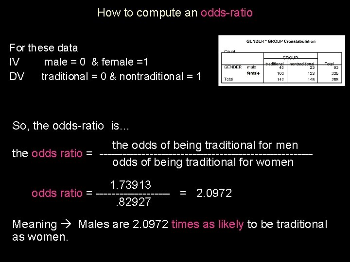
How to compute an odds-ratio For these data IV male = 0 & female =1 DV traditional = 0 & nontraditional = 1 So, the odds-ratio is… the odds of being traditional for men the odds ratio = ---------------------------odds of being traditional for women 1. 73913 odds ratio = ---------- = 2. 0972. 82927 Meaning Males are 2. 0972 times as likely to be traditional as women.

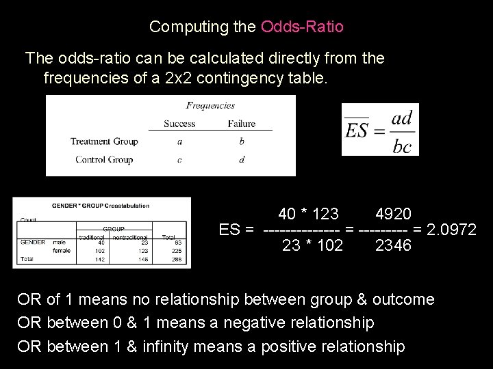
Computing the Odds-Ratio The odds-ratio can be calculated directly from the frequencies of a 2 x 2 contingency table. 40 * 123 4920 ES = ------- = 2. 0972 23 * 102 2346 OR of 1 means no relationship between group & outcome OR between 0 & 1 means a negative relationship OR between 1 & infinity means a positive relationship

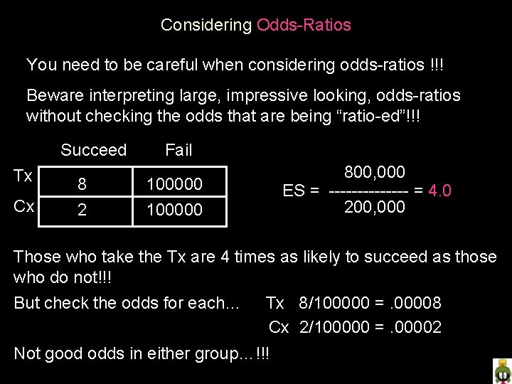
Considering Odds-Ratios You need to be careful when considering odds-ratios !!! Beware interpreting large, impressive looking, odds-ratios without checking the odds that are being “ratio-ed”!!! Succeed Tx Cx 8 2 Fail 800, 000 ES = ------- = 4. 0 200, 000 100000 Those who take the Tx are 4 times as likely to succeed as those who do not!!! But check the odds for each… Tx 8/100000 =. 00008 Cx 2/100000 =. 00002 Not good odds in either group…!!!

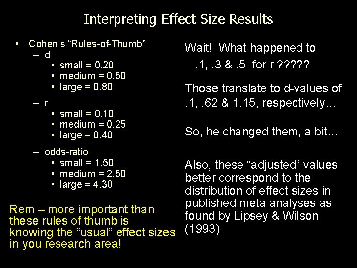
Interpreting Effect Size Results • Cohen’s “Rules-of-Thumb” – d • small = 0. 20 • medium = 0. 50 • large = 0. 80 – r • small = 0. 10 • medium = 0. 25 • large = 0. 40 – odds-ratio • small = 1. 50 • medium = 2. 50 • large = 4. 30 Wait! What happened to. 1, . 3 &. 5 for r ? ? ? Those translate to d-values of. 1, . 62 & 1. 15, respectively… So, he changed them, a bit… Also, these “adjusted” values better correspond to the distribution of effect sizes in published meta analyses as Rem – more important than found by Lipsey & Wilson these rules of thumb is knowing the “usual” effect sizes (1993) in you research area!

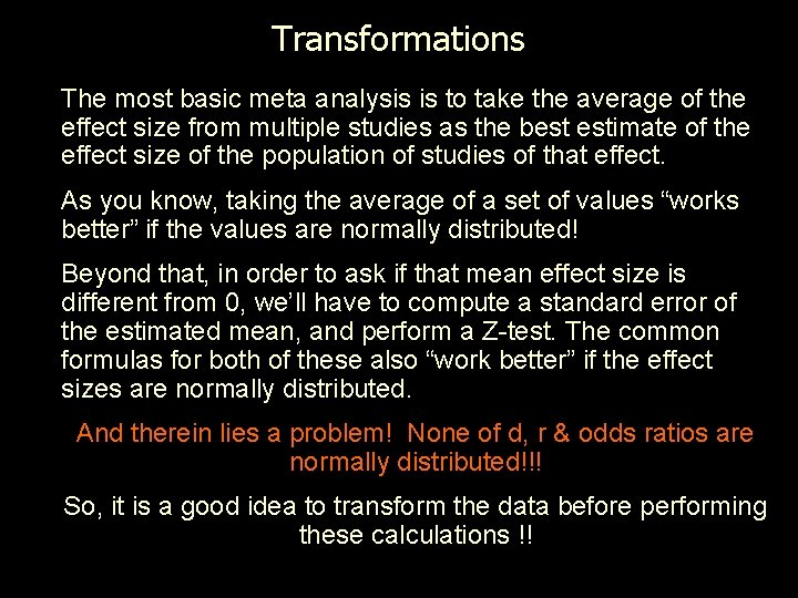
Transformations The most basic meta analysis is to take the average of the effect size from multiple studies as the best estimate of the effect size of the population of studies of that effect. As you know, taking the average of a set of values “works better” if the values are normally distributed! Beyond that, in order to ask if that mean effect size is different from 0, we’ll have to compute a standard error of the estimated mean, and perform a Z-test. The common formulas for both of these also “work better” if the effect sizes are normally distributed. And therein lies a problem! None of d, r & odds ratios are normally distributed!!! So, it is a good idea to transform the data before performing these calculations !!

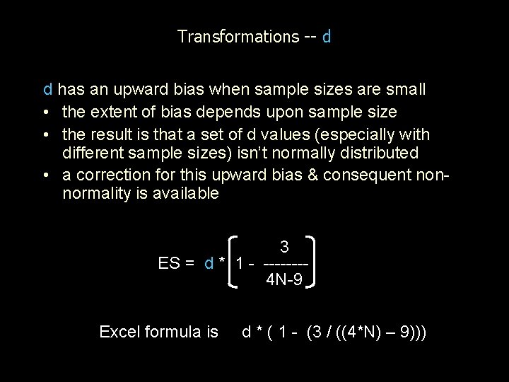
Transformations -- d d has an upward bias when sample sizes are small • the extent of bias depends upon sample size • the result is that a set of d values (especially with different sample sizes) isn’t normally distributed • a correction for this upward bias & consequent nonnormality is available 3 ES = d * 1 - -------4 N-9 Excel formula is d * ( 1 - (3 / ((4*N) – 9)))

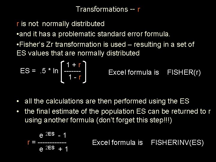
Transformations -- r r is not normally distributed • and it has a problematic standard error formula. • Fisher’s Zr transformation is used – resulting in a set of ES values that are normally distributed 1+r ES =. 5 * ln ------1 -r Excel formula is FISHER(r) • all the calculations are then performed using the ES • the final estimate of the population ES can be returned to r using another formula (don’t forget this step!!!) e 2 ES - 1 r = ------e 2 ES + 1 Excel formula is FISHERINV(ES)

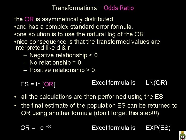
Transformations – Odds-Ratio the OR is asymmetrically distributed • and has a complex standard error formula. • one solution is to use the natural log of the OR • nice consequence is that the transformed values are interpreted like d & r – Negative relationship < 0. – No relationship = 0. – Positive relationship > 0. ES = ln [OR] Excel formula is LN(OR) • all the calculations are then performed using the ES • the final estimate of the population ES can be returned to OR using another formula (don’t forget this step!!!) OR = e ES Excel formula is EXP(ES)

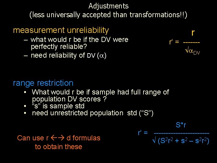
Adjustments (less universally accepted than transformations!!) measurement unreliability r – what would r be if the DV were perfectly reliable? – need reliability of DV ( ) r’ = ------ DV range restriction • What would r be if sample had full range of population DV scores ? • “s” is sample std • need unrestricted population std (“S”) Can use r d formulas to obtain these S*r r’ = ----------- (S 2 r 2 + s 2 – s 2 r 2)

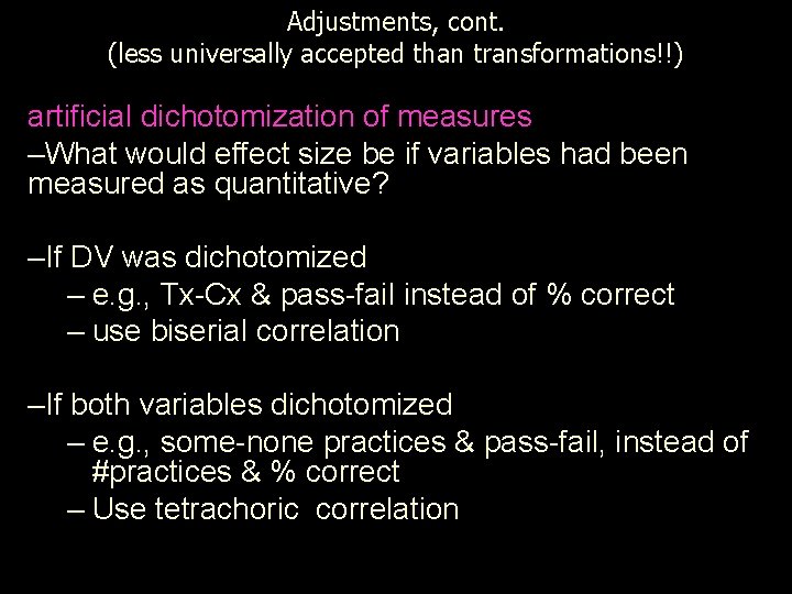
Adjustments, cont. (less universally accepted than transformations!!) artificial dichotomization of measures –What would effect size be if variables had been measured as quantitative? –If DV was dichotomized – e. g. , Tx-Cx & pass-fail instead of % correct – use biserial correlation –If both variables dichotomized – e. g. , some-none practices & pass-fail, instead of #practices & % correct – Use tetrachoric correlation

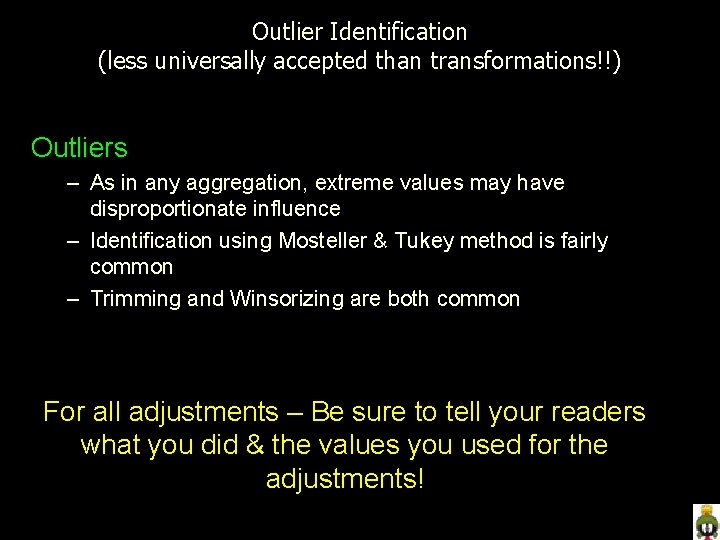
Outlier Identification (less universally accepted than transformations!!) Outliers – As in any aggregation, extreme values may have disproportionate influence – Identification using Mosteller & Tukey method is fairly common – Trimming and Winsorizing are both common For all adjustments – Be sure to tell your readers what you did & the values you used for the adjustments!