AP Statistics Quarterly 1 Review THE WEAKEST LINK

AP Statistics Quarterly 1 Review THE WEAKEST LINK: GET IN A GROUP OF 2 -3. MAKE A TEAM NAME, GET A COMMUNICATOR, ERASER, AND MARKER.

POINTS TEAM 1 TEAM 2 TEAM 3 TEAM 4 TEAM 5 TEAM 6 TEAM 7 TEAM 8 TEAM 9 TEAM 10 1 2 3 4 5 6 7 8 9 10 11 12 13 14 15 16 17 18

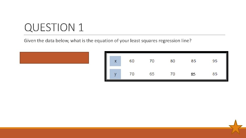
QUESTION 1 85

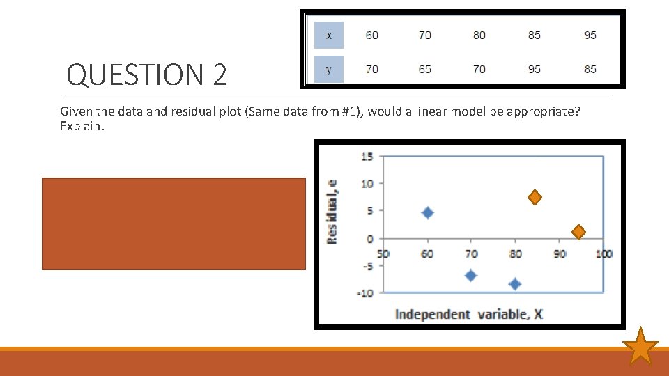
QUESTION 2 Given the data and residual plot (Same data from #1), would a linear model be appropriate? Explain. Yes, the residual plot shows a random scatter above and below The LSRL.

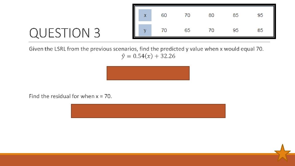
QUESTION 3

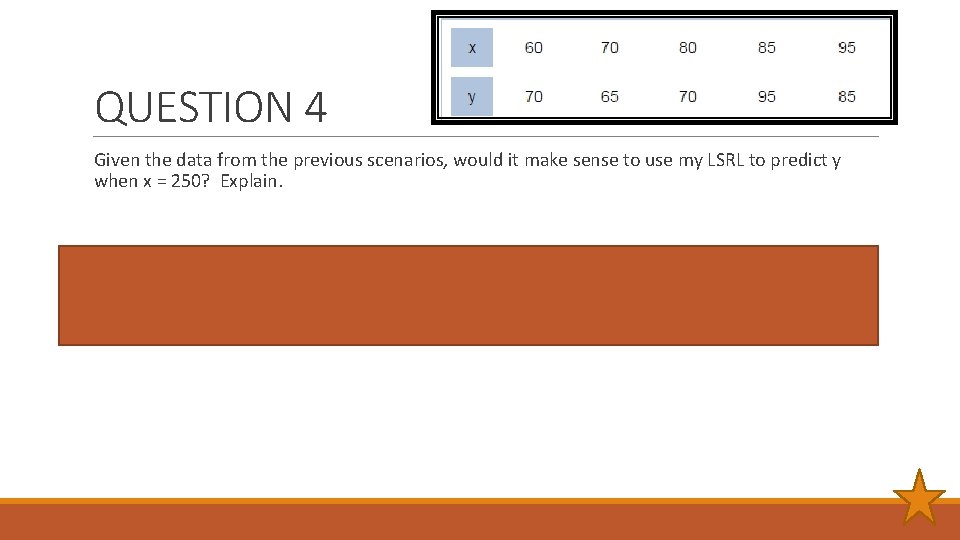
QUESTION 4 Given the data from the previous scenarios, would it make sense to use my LSRL to predict y when x = 250? Explain. No, that is extrapolation. The trend of the LSRL may not be relevant or make sense in context of the situation that far away from our given data.

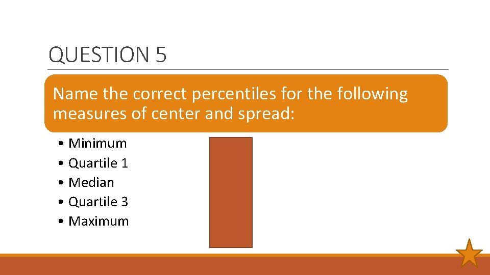
QUESTION 5 Name the correct percentiles for the following measures of center and spread: • Minimum • Quartile 1 • Median • Quartile 3 • Maximum 0 th 25 th 50 th 75 th 100 th

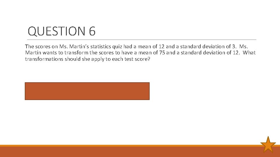
QUESTION 6 The scores on Ms. Martin’s statistics quiz had a mean of 12 and a standard deviation of 3. Ms. Martin wants to transform the scores to have a mean of 75 and a standard deviation of 12. What transformations should she apply to each test score? Multiply each score by 4 and add 27.

BONUS #1 (Will not count against your points) Name THIRTY Generation 1 Pokémon.

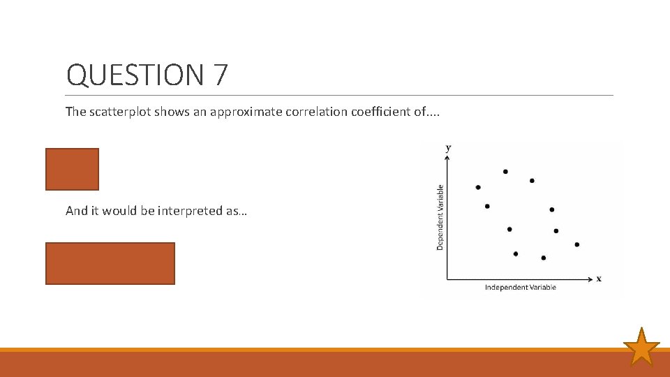
QUESTION 7 The scatterplot shows an approximate correlation coefficient of. . -0. 3 And it would be interpreted as… Weak Negative

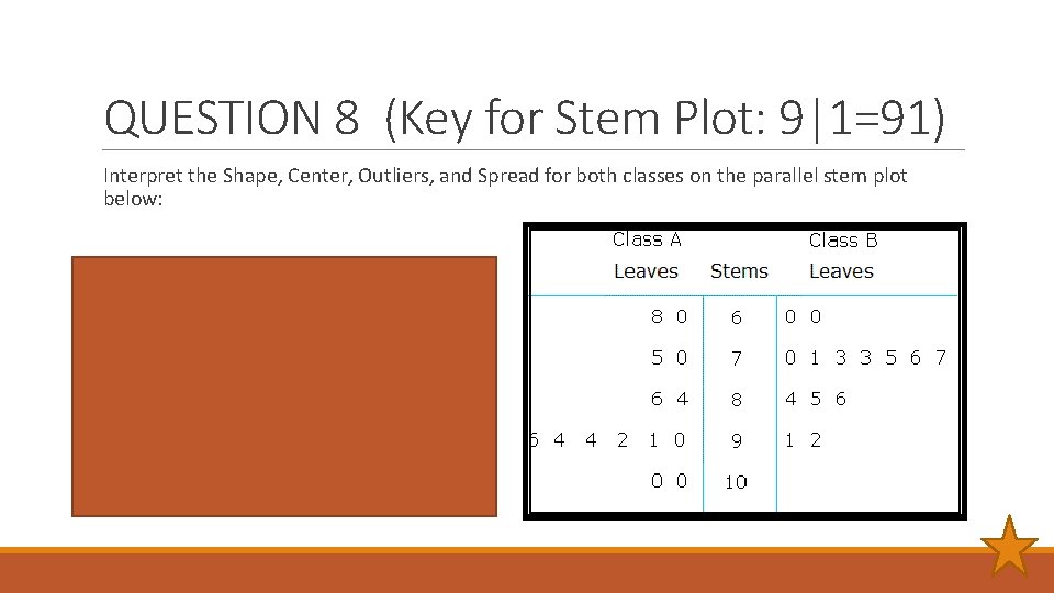
QUESTION 8 (Key for Stem Plot: 9|1=91) Interpret the Shape, Center, Outliers, and Spread for both classes on the parallel stem plot below: CLASS A CLASS B SKEWED NO OUTLIERS MED = 90. 5 MED = 75. 5 IQR = 19 IQR = 14

QUESTION 9 Scores on the Wechsler Adult Intelligence Scale (A standard IQ test) for the 20 – 34 age group are approximately Normally distributed with μ=110 and σ=25. ◦ What percent of people aged 20 – 34 have IQs between 125 and 150? ~21. 95% ◦ What percent of people aged 20 – 34 have IQs above 140? ~11. 51%

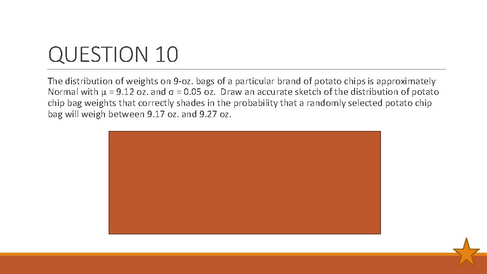
QUESTION 10 The distribution of weights on 9 -oz. bags of a particular brand of potato chips is approximately Normal with μ = 9. 12 oz. and σ = 0. 05 oz. Draw an accurate sketch of the distribution of potato chip bag weights that correctly shades in the probability that a randomly selected potato chip bag will weigh between 9. 17 oz. and 9. 27 oz.

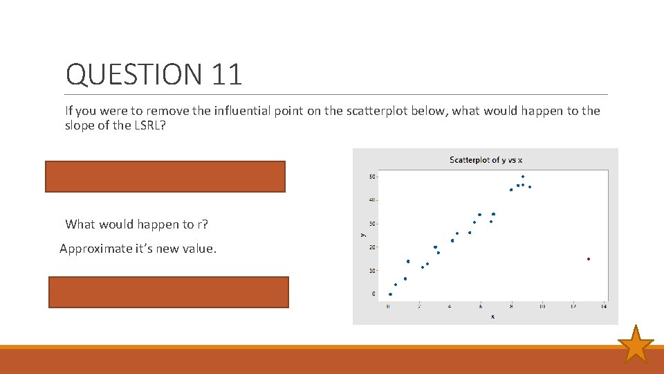
QUESTION 11 If you were to remove the influential point on the scatterplot below, what would happen to the slope of the LSRL? Slope will increase greatly. What would happen to r? Approximate it’s new value. r would increase to almost 1.

BONUS #2 (Will not count against your points) Can you name TEN counties in Maryland?

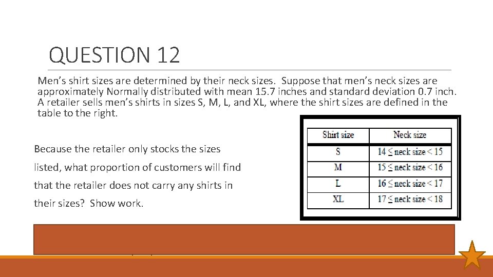
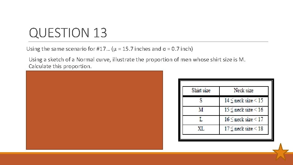
QUESTION 12 Men’s shirt sizes are determined by their neck sizes. Suppose that men’s neck sizes are approximately Normally distributed with mean 15. 7 inches and standard deviation 0. 7 inch. A retailer sells men’s shirts in sizes S, M, L, and XL, where the shirt sizes are defined in the table to the right. Because the retailer only stocks the sizes listed, what proportion of customers will find that the retailer does not carry any shirts in their sizes? Show work. P(X < 14) + P (X > 18) = 0. 008 + 0. 0006 = 0. 0086 or ~0. 86% of customers will find that the retailer does not carry any shirts in their sizes.

QUESTION 13 Using the same scenario for #17… (μ = 15. 7 inches and σ = 0. 7 inch) Using a sketch of a Normal curve, illustrate the proportion of men whose shirt size is M. Calculate this proportion. P(15 ≤ X < 16) = ~50. 72% of men have Medium shirt size.

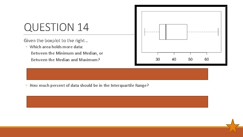
QUESTION 14 Given the boxplot to the right… ◦ Which area holds more data: Between the Minimum and Median, or Between the Median and Maximum? NEITHER. Both areas hold 50% of the data, even in skewed distributions. ◦ How much percent of data should be in the Interquartile Range? 50%. The central 50% specifically.

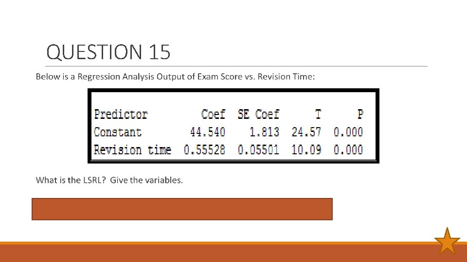
QUESTION 15

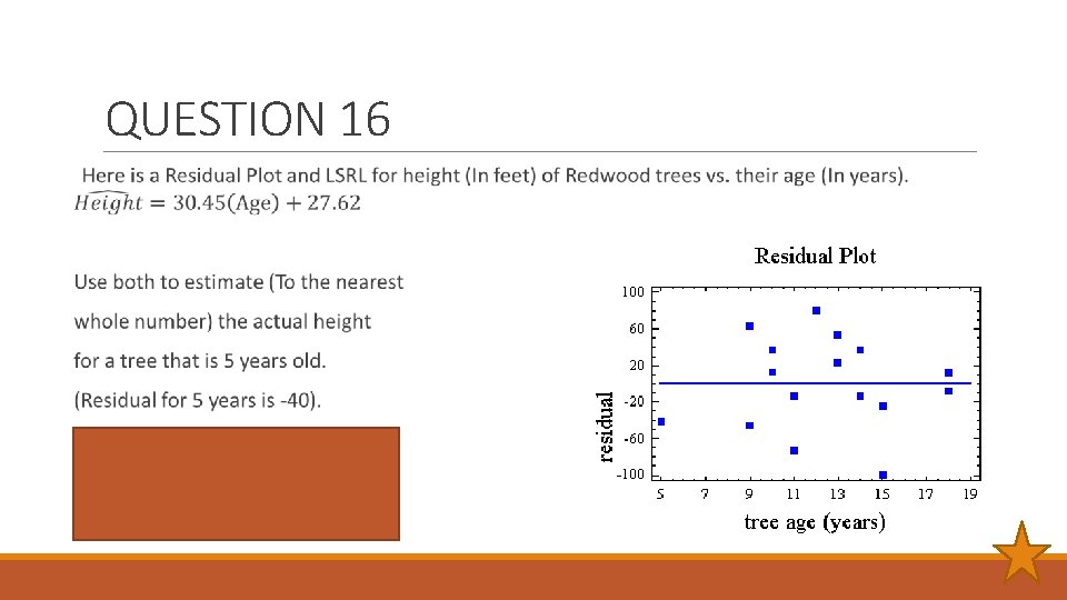
QUESTION 16

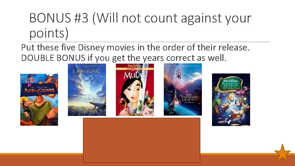
BONUS #3 (Will not count against your points) Put these five Disney movies in the order of their release. DOUBLE BONUS if you get the years correct as well. 1. 2. 3. 4. 5. Alice in Wonderland (1951) The Lion King (1994) Mulan (1998) The Emperor’s New Groove (2000) Treasure Planet (2002)

QUESTION 17 Put the following in order from least to greatest: ◦ ◦ ◦ V: The Median W: A z-score of -1. 00 X: The 80 th Percentile Y: Quartile 1 Z: A data point of 60 in a distribution that is approximately N(30, 15) W (16 th %ile), Y (25 th %ile), V (50 th %ile), X (80 th %ile), Z (97. 5%ile).

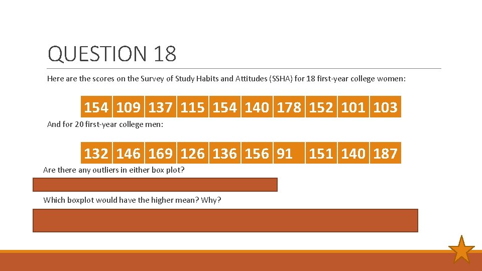
QUESTION 18 Here are the scores on the Survey of Study Habits and Attitudes (SSHA) for 18 first-year college women: 154 109 137 115 154 140 178 152 101 103 And for 20 first-year college men: 132 146 169 126 136 156 91 151 140 187 Are there any outliers in either box plot? Yes, The college men have an outlier of score 91. Which boxplot would have the higher mean? Why? The college men due to their boxplot being skewed more to the right than the college women’s boxplot.