Econometrics Econ 504 Chapter 11 Regression with Panel

Econometrics Econ. 504 Chapter 11: Regression with Panel Data

I. The Natural of Panel Data § Recall: data used to estimate and test your econometrics model is typically classified into one of the three possible types: Cross Sectional Data, Time Series Data, Panel Data. § In time series data we observe the values of one or more variables over a period of time (e. g. , GDP for several quarters or years). § In cross-section data, values of one or more variables are collected for several sample units, or subjects, at the same point in time (e. g. , crime rates for 50 states in the United States for a given year).

§ In panel data the same cross-sectional unit (say a family or a firm or a state) is surveyed over time. In short, panel data have space as well as time dimensions. § Recall: the error in each time period was assumed to be uncorrelated with the explanatory variables in the same time period. § However, for certain panel data applications this assumption is too strong. In fact a primary motivation for using panel data is to solve the omitted variables problem.

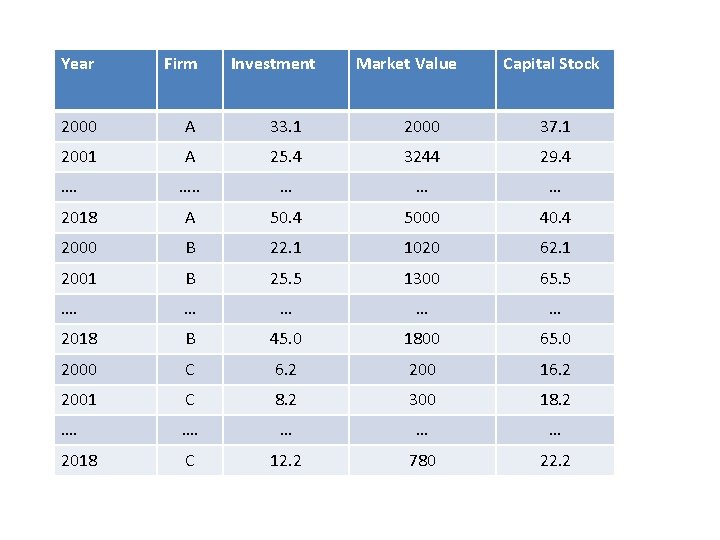
Example; • Table below gives data on investment, market value of the firm, and capital stock for three companies for the period 2000– 2018. • Assuming the sample of three companies combines of company A, B, and C.

Year Firm 2000 A 33. 1 2000 37. 1 2001 A 25. 4 3244 29. 4 …. . … … … 2018 A 50. 4 5000 40. 4 2000 B 22. 1 1020 62. 1 2001 B 25. 5 1300 65. 5 …. … … 2018 B 45. 0 1800 65. 0 2000 C 6. 2 200 16. 2 2001 C 8. 2 300 18. 2 …. … … … 2018 C 12. 2 780 22. 2 …. Investment Market Value Capital Stock

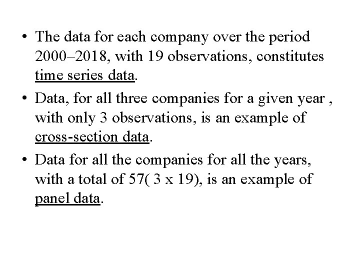
• The data for each company over the period 2000– 2018, with 19 observations, constitutes time series data. • Data, for all three companies for a given year , with only 3 observations, is an example of cross-section data. • Data for all the companies for all the years, with a total of 57( 3 x 19), is an example of panel data.

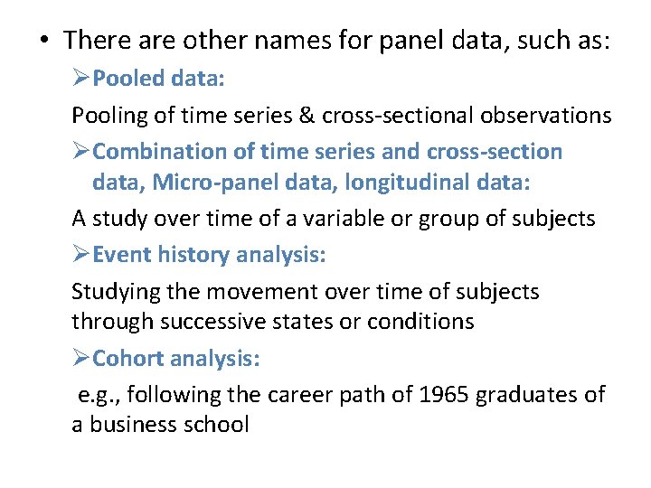
• There are other names for panel data, such as: ØPooled data: Pooling of time series & cross-sectional observations ØCombination of time series and cross-section data, Micro-panel data, longitudinal data: A study over time of a variable or group of subjects ØEvent history analysis: Studying the movement over time of subjects through successive states or conditions ØCohort analysis: e. g. , following the career path of 1965 graduates of a business school

• Although there are indirect variations between these different names, all these names essentially mean movement over time of crosssectional units. • Panel data is now being used increasingly in economic research.

II. Why Panel Approach § If data are not available from some of the variables, then they cannot be included in the regression and OLS estimators of the regression coefficients could have omitted variable bias. § Using panel approach would provide a method for controlling for some types of omitted variables without observing them. § However, in order to process such method, the data should be specified as a panel data.

• There advantages of panel data over crosssection or time series data. Baltagi (1995) lists the following: 1 - Since panel data relate to individuals, firms, states, countries, etc. , over time, there is bound to be heterogeneity in these units. The techniques of panel data estimation can take such heterogeneity explicitly into account by allowing for subjectspecific variables.

2 - By combining time series of cross-section observations, panel data gives “more informative data, more variability, less collinearity among variables, more degrees of freedom and more efficiency. ” 3 - By studying the repeated cross section of observations, panel data are better suited to study the dynamics of change.

4 - Panel data can better detect and measure effects that simply cannot be observed in pure cross-section or pure time series data. 5 - Panel data enables us to study more complicated behavioral models. 6 - By making data available for several thousand units, panel data can minimize the bias that might result if we aggregate individuals or firms into broad aggregates.

Recall our last Example: § The panel data in our example is called a balanced panel; a panel is said to be balanced if each subject (firm, individuals, etc. ) has the same number of observations. § Note that if each entity has a different number of observations, then we have an unbalanced panel. § Accordingly, to estimate the panel data, there are four possibilities: 1. Pooled OLS model: We simply pool all 57 observations and estimate a “grand” regression, neglecting the cross-section and time series nature of our data.

2. The fixed effects least squares dummy variable (LSDV) model: Here we pool all 57 observations, but allow each crosssection unit (i. e. , company in our example) to have its own (intercept) dummy variable. 3. The fixed effects time model: Here also we pool all 57 observations, but for each company with time effect. Such way would allow for time effect if we believe that the estimated function changes over time

4. The random effects model: Unlike the LSDV model, in which we allow each company to have its own (fixed) intercept value, we assume that the intercept values are a random drawing from a much bigger population of airlines.

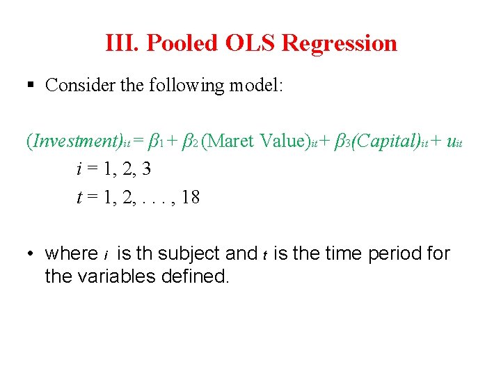
III. Pooled OLS Regression § Consider the following model: (Investment)it = β 1 + β 2 (Maret Value)it + β 3(Capital)it + uit i = 1, 2, 3 t = 1, 2, . . . , 18 • where i is th subject and t is the time period for the variables defined.

• Notice that we have pooled together all 57 observations, but note that we are assuming the regression coefficients are the same for all the company. • That is, there is no distinction between the company, one company is as good as the other. • Such assumption may be difficult to maintain.

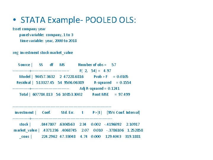
• STATA Example- POOLED OLS: tsset company year panel variable: company, 1 to 3 time variable: year, 2000 to 2018 reg investment stock market_value Source | SS df MS Number of obs = 57 -------+---------------F( 2, 54) = 4. 97 Model | 94457. 3632 2 47228. 6816 Prob > F = 0. 0105 Residual | 513327. 45 54 9506. 06389 R-squared = 0. 1554 -------+---------------Adj R-squared = 0. 1241 Total | 607784. 813 56 10853. 3002 Root MSE = 97. 499 ---------------------------------------investment | Coef. Std. Err. t P>|t| [95% Conf. Interval] -------+--------------------------------stock |. 8447807. 6306563 2. 34 0. 002 -. 4196092 2. 10917 market_value |. 4371236. 4068745 2. 07 0. 010 -. 3786106 1. 252858 _cons | 224. 2962 47. 33048 4. 74 0. 000 129. 4043 319. 1881

Problems with this model • The major problem with this model is that it does not distinguish between the various companies nor does it tell us whether the response of investment (DV) to the explanatory variables (IV’s) over time is the same for all the companies. • In other words, by lumping together different companies at different times we hide the heterogeneity (individuality or uniqueness) that may exist among the companies.

• Another way of stating this is that the individuality of each subject (company) is included in the disturbance term uit. • As a consequence, it is quite possible that the error term may be correlated with some of the regressors included in the model. • If that is the case, then estimated coefficients may be biased as well as inconsistent.

Dealing with this model • Recall that one of the important assumptions of the classical linear regression model is that there is no correlation between the regressors and the disturbance or error term. • Now…Broadly Speaking… Think of a variable that is related to the company’s investment ( such as management quality) where this additional variable “management quality” is a time invariant variable ( does not change over time).

• Of the variables included in the model, only the variable “management quality” is time-invariant (or time-constant) because it varies among subjects (companies) but is constant over time for a given subject (company). • Although it is time-invariant, the variable “management quality” is not directly observable and therefore we cannot measure its contribution to the investment function.

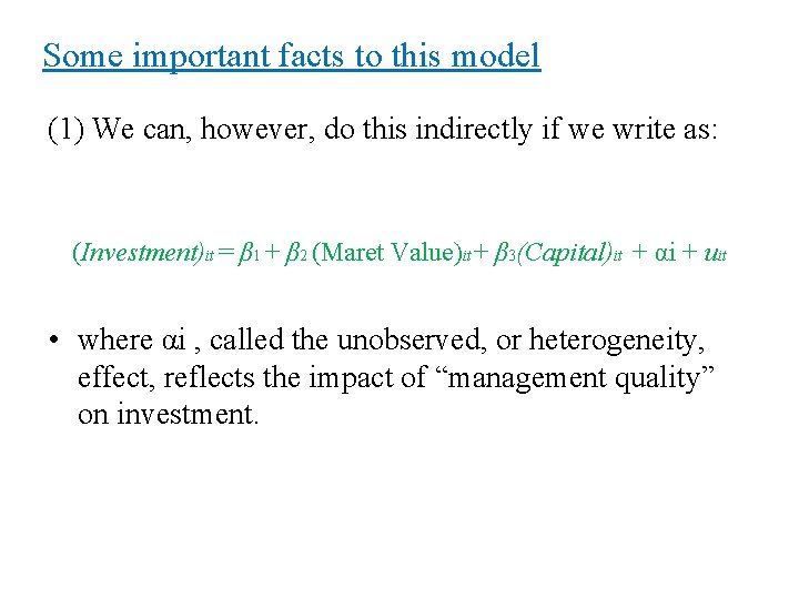
Some important facts to this model (1) We can, however, do this indirectly if we write as: (Investment)it = β 1 + β 2 (Maret Value)it + β 3(Capital)it + αi + uit • where αi , called the unobserved, or heterogeneity, effect, reflects the impact of “management quality” on investment.

• Note that for simplicity we have shown only the unobserved effect of “management quality”, but in reality there may be more such unobserved effects, for example, the nature of ownership (privately owned or publicly owned), whether it is a minorityowned company, whether the CEO is a man or a woman, etc. • Although such variables may differ among the subjects (companies), they will probably remain the same for any given subject over the sample period.

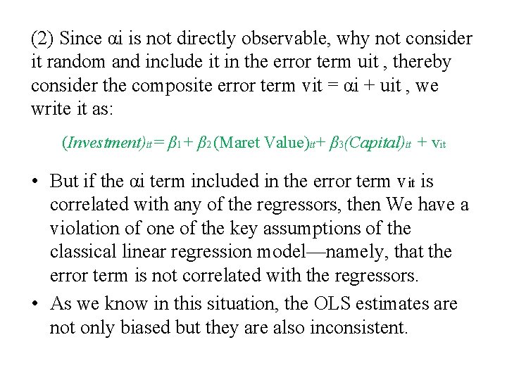
(2) Since αi is not directly observable, why not consider it random and include it in the error term uit , thereby consider the composite error term vit = αi + uit , we write it as: (Investment)it = β 1 + β 2 (Maret Value)it + β 3(Capital)it + vit • But if the αi term included in the error term vit is correlated with any of the regressors, then We have a violation of one of the key assumptions of the classical linear regression model—namely, that the error term is not correlated with the regressors. • As we know in this situation, the OLS estimates are not only biased but they are also inconsistent.

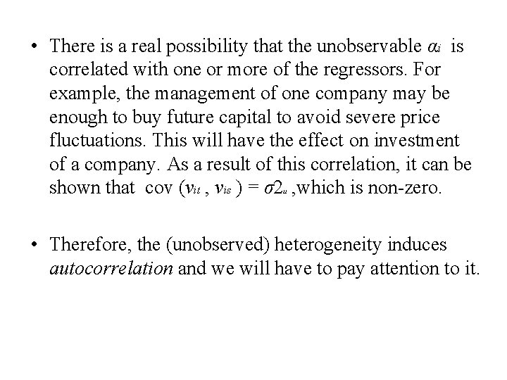
• There is a real possibility that the unobservable αi is correlated with one or more of the regressors. For example, the management of one company may be enough to buy future capital to avoid severe price fluctuations. This will have the effect on investment of a company. As a result of this correlation, it can be shown that cov (vit , vis ) = σ2 , which is non-zero. u • Therefore, the (unobserved) heterogeneity induces autocorrelation and we will have to pay attention to it.

• The question, therefore, is how we account for the unobservable, or heterogeneity, effect(s) so that we can obtain consistent and/or efficient estimates of the parameters of the variables of prime interest. • Our prime interest may not be in obtaining the impact of the unobservable variables because they remain the same for a given subject. That is why such unobservable, or heterogeneity, effects are called nuisance parameters.

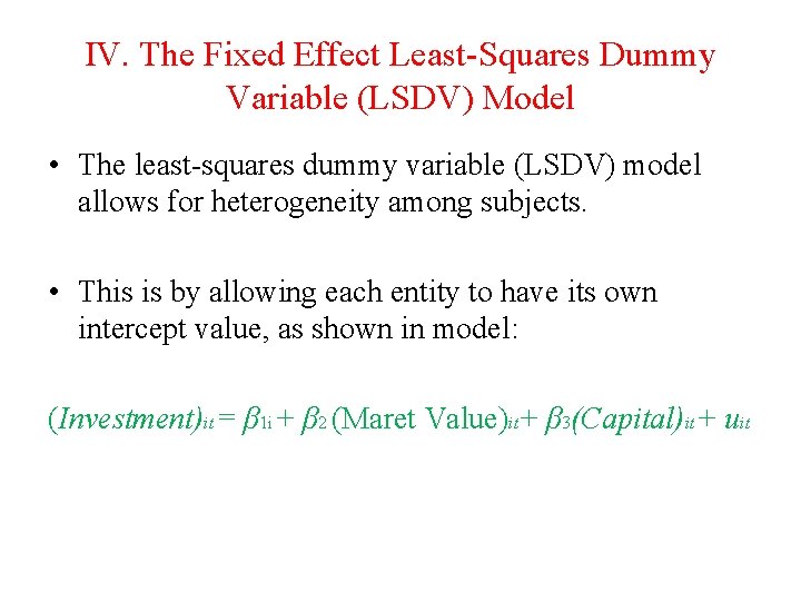
IV. The Fixed Effect Least-Squares Dummy Variable (LSDV) Model • The least-squares dummy variable (LSDV) model allows for heterogeneity among subjects. • This is by allowing each entity to have its own intercept value, as shown in model: (Investment)it = β 1 i + β 2 (Maret Value)it + β 3(Capital)it + uit

• Note the subscript i is now on the intercept term to suggest that the intercepts of the three companies may be different. • The difference may be due to special features of each company, such as managerial style, managerial quality, or the type of market sector each company is serving. • This model is known as the fixed effects (regression) model (FEM).

• The term “fixed effects” is due to the fact that, although the intercept may differ across subjects (here three companies), each entity’s intercept does not vary over time, that is, it is time-invariant. • Notice that if we were to write the intercept as β 1 it , it would suggest that the intercept of each entity or individual is time-variant. It may be noted that the FEM given assumes that the (slope) coefficients of the regressors do not vary across individuals or over time.

How do we actually allow for the (fixed effect) intercept to vary among the companies? • We can easily do this by using the dummy variable technique, particularly the differential intercept dummy technique, Now we write the model as: (Investment)it = α 1 + α 2 D 2 i + α 3 D 3 i + β 2 (Maret Value)it + β 3(Capital)it + uit where (D 2 i = 1 for company 2, 0 otherwise); (D 3 i = 1 for company 3, 0 otherwise).

• Notice that since we have three companies, we have introduced only two dummy variables to avoid falling into the dummy-variable trap (i. e. , the situation of perfect collinearity). • Here we are treating company (1) as the base, or reference, category. Of course, you can choose any company as the reference point.

• As a result, the intercept “α 1 “ is the intercept value of company (1) and the other “α” coefficients represent by how much the intercept values of the other company differ from the intercept value of the first airline. • Thus, α 2 tells by how much the intercept value of the second company differs from α 1. The sum (α 1 + α 2) gives the actual value of the intercept for company (2). The intercept values of the other company (third one) can be computed similarly. • Keep in mind that if you want to introduce a dummy for each company , you will have to drop the (common) intercept; otherwise, you will fall into the dummy-variable trap.

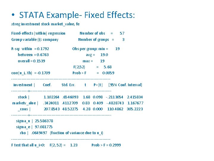
• STATA Example- Fixed Effects: xtreg investment stock market_value, fe Fixed-effects (within) regression Group variable (i): company R-sq: within = 0. 1792 between = 0. 6763 overall = 0. 1539 Number of obs = Number of groups = 57 3 Obs per group: min = 19 avg = 19. 0 max = 19 F(2, 52) = 5. 68 corr(u_i, Xb) = -0. 1709 Prob > F = 0. 0059 ---------------------------------------investment | Coef. Std. Err. t P>|t| [95% Conf. Interval] -------+--------------------------------stock | 1. 102264. 6546093 1. 68 0. 098 -. 2113054 2. 415834 marketv_alue |. 3424011. 4112709 0. 83 0. 409 -. 4828743 1. 167677 _cons | 207. 8543 48. 52275 4. 28 0. 000 110. 4862 305. 2223 -------+--------------------------------sigma_u | 25. 586378 sigma_e | 97. 081775 rho |. 0649497 (fraction of variance due to u_i) ---------------------------------------F test that all u_i=0: F(2, 52) = 1. 23 Prob > F = 0. 2999

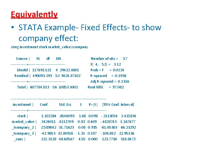
Equivalently • STATA Example- Fixed Effects- to show company effect: xireg investment stock market_value i. company Source | SS df MS -------+---------------Model | 117691. 521 4 29422. 8801 Residual | 490093. 293 52 9424. 87102 -------+---------------Total | 607784. 813 56 10853. 3002 Number of obs = 57 F( 4, 52) = 3. 12 Prob > F = 0. 0224 R-squared = 0. 1936 Adj R-squared = 0. 1316 Root MSE = 97. 082 ---------------------------------------investment | Coef. Std. Err. t P>|t| [95% Conf. Interval] -------+--------------------------------stock | 1. 102264. 6546093 1. 68 0. 098 -. 2113054 2. 415834 market_value |. 3424011. 4112709 0. 83 0. 409 -. 4828743 1. 167677 _Icompany_2 | 2. 589642 31. 71623 0. 08 0. 935 -61. 05363 66. 23292 _Icompany_3 | -42. 9653 32. 84916 -1. 31 0. 197 -108. 882 22. 95136 _cons | 221. 3128 48. 60567 4. 55 0. 000 123. 7784 318. 8472

IIV. The Fixed-Effect Model, Time Effect • The estimated model is known as a one-way fixed effects model because we have allowed the intercepts to differ between companies. • But we can also allow for time effect if we believe that the investment function changes over time because of factors such as technological changes, changes in government regulation and/or tax policies, and other such effects. • Such a time effect can be easily accounted for if we introduce time dummies, one for each year from 2000 to 2018.

• If we do that, the model that emerges is called a twoway fixed effects model because we have allowed for both individual and time effects. • In the present example, if we add the time dummies, we will have in all 24 coefficients to estimate—the common intercept, 2 company dummies, 19 time dummies, and 2 slope coefficients. • As you can see, we will consume several degrees of freedom.

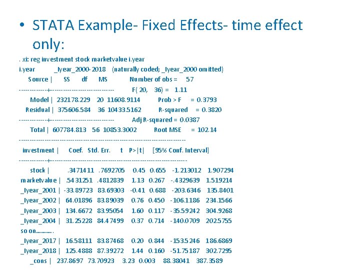
• STATA Example- Fixed Effects- time effect only: . xi: reg investment stock marketvalue i. year _Iyear_2000 -2018 (naturally coded; _Iyear_2000 omitted) Source | SS df MS Number of obs = 57 -------+---------------F( 20, 36) = 1. 11 Model | 232178. 229 20 11608. 9114 Prob > F = 0. 3793 Residual | 375606. 584 36 10433. 5162 R-squared = 0. 3820 -------+---------------Adj R-squared = 0. 0387 Total | 607784. 813 56 10853. 3002 Root MSE = 102. 14 ---------------------------------------investment | Coef. Std. Err. t P>|t| [95% Conf. Interval] -------+--------------------------------stock |. 3471411. 7692705 0. 45 0. 655 -1. 213012 1. 907294 marketvalue |. 5431251. 4812839 1. 13 0. 267 -. 4329639 1. 519214 _Iyear_2001 | -33. 89723 83. 69303 -0. 41 0. 688 -203. 6346 135. 8401 _Iyear_2002 | 64. 01896 83. 89039 0. 76 0. 450 -106. 1186 234. 1566 _Iyear_2003 | 134. 6672 83. 95054 1. 60 0. 117 -35. 59242 304. 9268 _Iyear_2004 | 31. 25228 84. 47499 0. 37 0. 714 -140. 0709 202. 5755 so on………. . _Iyear_2017 | 16. 58111 83. 87468 0. 20 0. 844 -153. 5246 186. 6869 _Iyear_2018 | 125. 4888 87. 39272 1. 44 0. 160 -51. 75187 302. 7295 _cons | 237. 8697 73. 70923 3. 23 0. 003 88. 38041 387. 3589

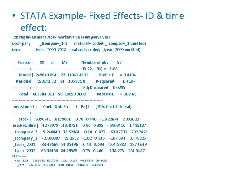
• STATA Example- Fixed Effects- ID & time effect: . xi: reg investment stock marketvalue i. company i. year i. company _Icompany_1 -3 (naturally coded; _Icompany_1 omitted) i. year _Iyear_2000 -2018 (naturally coded; _Iyear_2000 omitted) Source | SS df MS Number of obs = 57 -------+---------------F( 22, 34) = 1. 08 Model | 249643. 094 22 11347. 4133 Prob > F = 0. 4134 Residual | 358141. 72 34 10533. 58 R-squared = 0. 4107 -------+---------------Adj R-squared = 0. 0295 Total | 607784. 813 56 10853. 3002 Root MSE = 102. 63 ---------------------------------investment | Coef. Std. Err. t P>|t| [95% Conf. Interval] -------+--------------------------------stock |. 6396741. 8179861 0. 78 0. 440 -1. 022674 2. 302022 marketvalue |. 4273979. 4958751 0. 86 0. 395 -. 5803416 1. 435137 _Icompany_2 | 5. 248443 33. 62084 0. 16 0. 877 -63. 07732 73. 57421 _Icompany_3 | -35. 86087 35. 2532 -1. 02 0. 316 -107. 504 35. 78225 _Iyear_2001 | -33. 43664 84. 09496 -0. 40 0. 693 -204. 3382 137. 4649 _Iyear_2002 | 63. 03436 84. 29565 0. 75 0. 460 -108. 275 234. 3437 So on……… _Iyear_2018 | 115. 5368 88. 27149 1. 31 0. 199 -63. 85242 294. 9261 _cons | 232. 3339 75. 03293 3. 10 0. 004 79. 84861 384. 8191

• Furthermore, if we decide to allow the slope coefficients to differ among the companies, we can interact the two firm (company) dummies with each of the two explanatory variables and introduce differential slope dummy coefficients. Then we will have to estimate 4 additional coefficients (two dummies interacted with two explanatory variables). • As if this is not enough, if we interact the 19 time dummies with the two explanatory variables, we will have in all 38 additional coefficients to estimate. • As you can see, we will not have any degrees of freedom left.

Caution in the Use of the Fixed Effect Model • First, if you introduce too many dummy variables, you will run up against the degrees of freedom problem. • Second, with many dummy variables in the model, both individual and interactive or multiplicative, there is always the possibility of multicollinearity, which might make precise estimation of one or more parameters difficult. • Third, in some situations the LSDV may not be able to identify the impact of time invariant variables.

V. The Random-Effects Model • The important question is whether the inclusion of the dummy variables—and the consequent loss of the number of degrees of freedom—is really necessary. • The reasoning underlying the covariance model is that in “specifying the regression model we have failed to include relevant explanatory variables that do not change over time”. • Also possibly others that do change over time but have the same value for all cross-sectional units. • That the inclusion of dummy variables is a cover up of our ignorance.

• If the dummy variables do in fact represent a lack of knowledge about the (true) model, why not express this ignorance through the disturbance term? . • This is precisely the approach suggested by the proponents of the so-called error components model (ECM) or random effects model (REM), which we will now illustrate with our investment function.

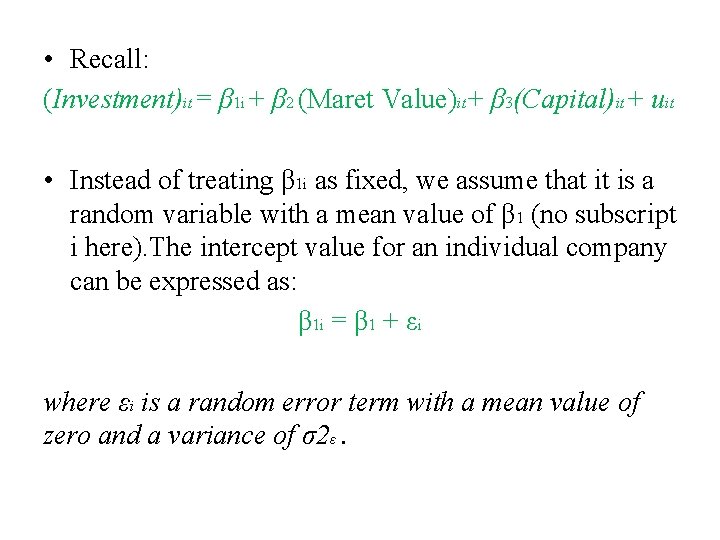
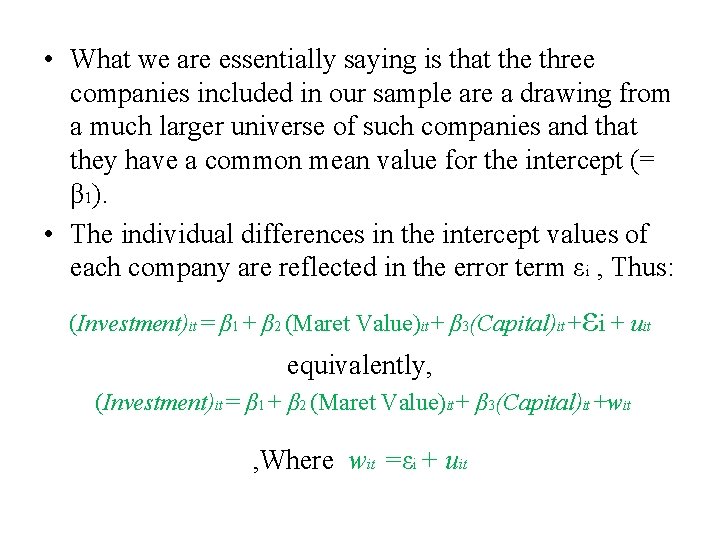
• Recall: (Investment)it = β 1 i + β 2 (Maret Value)it + β 3(Capital)it + uit • Instead of treating β 1 i as fixed, we assume that it is a random variable with a mean value of β 1 (no subscript i here). The intercept value for an individual company can be expressed as: β 1 i = β 1 + εi where εi is a random error term with a mean value of zero and a variance of σ2ε.

• What we are essentially saying is that the three companies included in our sample are a drawing from a much larger universe of such companies and that they have a common mean value for the intercept (= β 1). • The individual differences in the intercept values of each company are reflected in the error term εi , Thus: ε (Investment)it = β 1 + β 2 (Maret Value)it + β 3(Capital)it + i + uit equivalently, (Investment)it = β 1 + β 2 (Maret Value)it + β 3(Capital)it +wit , Where wit =εi + uit

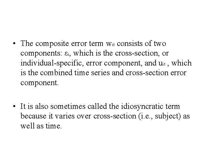
• The composite error term wit consists of two components: εi, which is the cross-section, or individual-specific, error component, and uit , which is the combined time series and cross-section error component. • It is also sometimes called the idiosyncratic term because it varies over cross-section (i. e. , subject) as well as time.

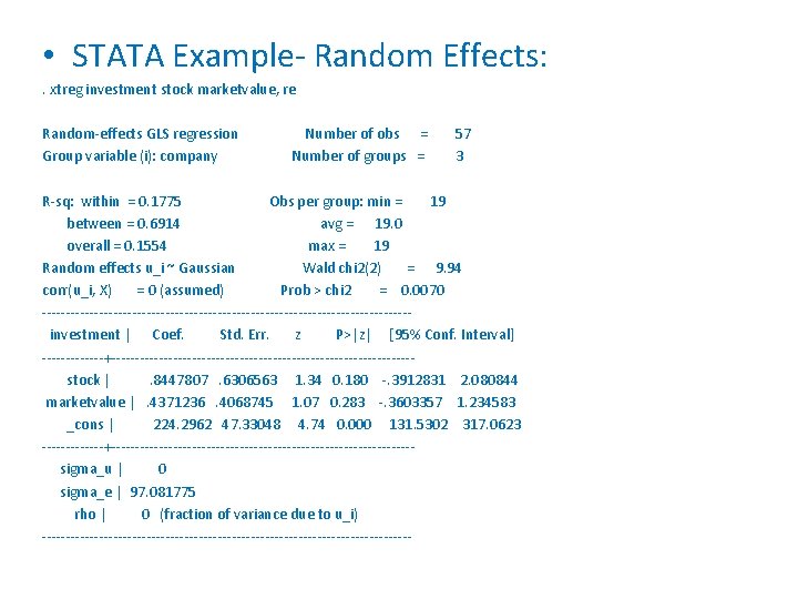
• STATA Example- Random Effects: . xtreg investment stock marketvalue, re Random-effects GLS regression Group variable (i): company Number of obs = Number of groups = 57 3 R-sq: within = 0. 1775 Obs per group: min = 19 between = 0. 6914 avg = 19. 0 overall = 0. 1554 max = 19 Random effects u_i ~ Gaussian Wald chi 2(2) = 9. 94 corr(u_i, X) = 0 (assumed) Prob > chi 2 = 0. 0070 ---------------------------------------investment | Coef. Std. Err. z P>|z| [95% Conf. Interval] -------+--------------------------------stock |. 8447807. 6306563 1. 34 0. 180 -. 3912831 2. 080844 marketvalue |. 4371236. 4068745 1. 07 0. 283 -. 3603357 1. 234583 _cons | 224. 2962 47. 33048 4. 74 0. 000 131. 5302 317. 0623 -------+--------------------------------sigma_u | 0 sigma_e | 97. 081775 rho | 0 (fraction of variance due to u_i) ---------------------------------------

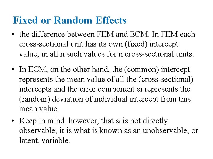
Fixed or Random Effects • the difference between FEM and ECM. In FEM each cross-sectional unit has its own (fixed) intercept value, in all n such values for n cross-sectional units. • In ECM, on the other hand, the (common) intercept represents the mean value of all the (cross-sectional) intercepts and the error component εi represents the (random) deviation of individual intercept from this mean value. • Keep in mind, however, that εi is not directly observable; it is what is known as an unobservable, or latent, variable.

VI. The Hausman test • If you compare the results of the fixed-effect and random-effect regressions, you will see that there are substantial differences between the two. • The important question now is: Which results are reliable? Or, to put it differently, which should be the choice between the two models? • We can apply the Hausman test to shed light on this question. • The null hypothesis underlying the Hausman test is that the FEM and ECM estimators do not differ substantially.

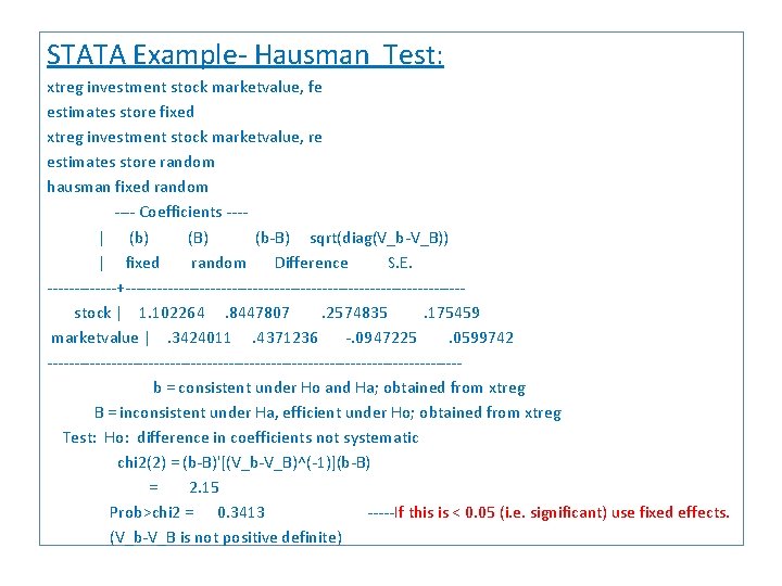
• The test statistic developed by Hausman has an asymptotic χ2 distribution. • If the null hypothesis is rejected, the conclusion is that the ECM is not appropriate because the random effects are probably correlated with one or more regressors. • In this case, FEM is preferred to ECM.

STATA Example- Hausman Test: xtreg investment stock marketvalue, fe estimates store fixed xtreg investment stock marketvalue, re estimates store random hausman fixed random ---- Coefficients ---| (b) (B) (b-B) sqrt(diag(V_b-V_B)) | fixed random Difference S. E. -------+--------------------------------stock | 1. 102264. 8447807. 2574835. 175459 marketvalue |. 3424011. 4371236 -. 0947225. 0599742 ---------------------------------------b = consistent under Ho and Ha; obtained from xtreg B = inconsistent under Ha, efficient under Ho; obtained from xtreg Test: Ho: difference in coefficients not systematic chi 2(2) = (b-B)'[(V_b-V_B)^(-1)](b-B) = 2. 15 Prob>chi 2 = 0. 3413 -----If this is < 0. 05 (i. e. significant) use fixed effects. (V_b-V_B is not positive definite)