Econometrics II ECON 2062 1 Regression Analysis with

Econometrics II ECON 2062 1. Regression Analysis with Qualitative Information: Binary (or Dummy Variables) 2. Introduction to Basic Regression Analysis with Time Series Data 3. Introduction to Simultaneous Equation models 4. Introduction to Panel Data Regression Models 2/12/2022 By: Wondimu E. 1

Dummy Variables • Qualitative variables which take one of two (1 or 0) values are known as dummy variables. Alternative names are indicator variables, binary variables, categorical variables, and dichotomous variables. • Typical examples include: gender, race, religion, marital status, etc. that is: Ø male (= 1 if are male, 0 otherwise), black (= 1 if it is black, 0 otherwise (white)), etc. 2/12/2022 By: Wondimu E. 2

• 2/12/2022 By: Wondimu E. 3

1. 2. 1. Dummy as Independent Variable A. Intercept Dummy Variables • Consider a simple model with one continuous variable (x) and one dummy (d) y = b 0 + d 0 d + b 1 x + u This can be interpreted as an intercept shift If d = 0, then y = b 0 + b 1 x + u If d = 1, then y = (b 0 + d 0) + b 1 x + u The case of d = 0 is the base group 2/12/2022 By: Wondimu E. 4

Example of d 0 > 0 y y = ( b 0 + d 0) + b 1 x d=1 { slope = b 1 d=0 b } 0 y = b 0 + b 1 x d 0 is known differential intercept coefficient 2/12/2022 By: Wondimu E. x 5

B. Slope Dummy Variables Yi = 1 + 2 Xi + 3 Di. Xi + Ui Yt Yi = 1 + ( 2 + 3)Xi + Ui 3 + 2 Yi = 1 + 2 Xi + U i 2 1 Xt 2/12/2022 By: Wondimu E. 6

C. Different Intercepts & Slopes Yi = 1 + 2 Xi + 3 Di + 4 Di. Xi + Ui Male: Di = 1 Yi Wage Female: Di = 0 Yi = ( 1 + 3) + ( 2 + 4)Xi + Ui Male 2+ 4 Yi = 1+ 2 Xi + Ui 1 + 3 1 2 Experience 2/12/2022 By: Wondimu E. Female Xi 7

1. 2. 2. Dummy Variables with More than Two Categories If a qualitative variable has m categories: • Introduce all m categories and drop the intercept term • Keep the intercept and introduce m-1 categories • If we do not follow the above guidelines then we fall into what is known as the dummy variable trap (perfect multicollinearity). 2/12/2022 By: Wondimu E. 8

For example, suppose we wish to test whether attendance at football matches is affected by the day the game is played. In this case there are seven categories (representing the days of the week), Therefore we should include six dummy variables into our estimated model Where, for example, D 1 = 1 if match was played on a Sunday; = 0 otherwise. 2/12/2022 By: Wondimu E. 9

C. The use of dummy variables in seasonal analysis • Many economic time series based on monthly or quarterly data exhibit seasonal patterns (regular oscillatory movement). Examples are sales of department stores at Christmas time, demand for money (cash balances) by households at holiday times, demand for ice cream and soft drinks during the summer, etc. • Often it is desirable to remove the seasonal factor, or component, from a time series so that one may concentrate on the other components, such as the trend. 2/12/2022 By: Wondimu E. 10

1. Regression with a Binary Dependent Variable So far the dependent variable (Y) has been continuous: • district-wide average test score • traffic fatality rate • Personal consumption expenditure etc… What if Y is binary? • Suppose we want to study the labor-force participation of adult males as a function of the unemployment rate, average wage rate, family income, education, etc. A person either is in the labor force or not. • A family may or may not own a house. If it owns a house, it takes a value 1 and 0 if it does not. 2/12/2022 By: Wondimu E. 11

• Four most commonly used approaches to estimating binary response models (type of binomial models). A. Linear probability models B. Non-linear (index) models 2/12/2022 i. The logit model ii. The probit model By: Wondimu E. 7. 12

A. The Linear Probability Model • 2/12/2022 By: Wondimu E. 13

• 2/12/2022 By: Wondimu E. 14

2/12/2022 Yi Prob. 1 Pi 0 1 -Pi Total 1 By: Wondimu E. 15

• 2/12/2022 By: Wondimu E. 16

Example: linear probability model, HMDA data Mortgage denial v. ratio of debt payments to income (P/I ratio) in the HMDA data set 2/12/2022 By: Wondimu E. 17

Linear probability model: HMDA data • What is the predicted value for P/I ratio = 0. 3? • Calculating “effects”: increase P/I ratio from. 3 to. 4: • The effect on the probability of denial of an increase in P/I ratio from. 3 to. 4 is to increase the probability by. 061, that is, by 6. 1 percentage points. 2/12/2022 By: Wondimu E. 18

Next include black as a regressor: • Predicted probability of denial: for black applicant with P/I ratio =. 3: • for white applicant with P/I ratio =. 3: • difference =. 177 = 17. 7 percentage points. • Coefficient on black is significant at the 5% level. 2/12/2022 By: Wondimu E. 19

Problems with the LPM 2/12/2022 By: Wondimu E. 20

2/12/2022 By: Wondimu E. 21

IV. Functional Form: • Since the model is linear, a unit increase in X results in a constant change of in the probability of an event, holding all other variables constant. It means that, (∂P(y=1⁄xi))/∂x=β • Thus, the increase is the same regardless of the current value of X. In many applications, this is unrealistic. When the outcome is a probability, it is often substantively reasonable that the effects of independent variables will have diminishing returns as the predicted probability approaches 0 or 1. 2/12/2022 By: Wondimu E. 22

V. Questionable value of R 2 as a measure of goodness of fit. • For a given X, the Y values will be either 0 or 1. Therefore, all the Y values will either lie along the X-axis or along the line corresponding to 1. Therefore, generally no LPM is expected to fit such a scatter so well. As a result, the conventionally computed R 2 is likely to be much lower than 1 for such models. • Aldrich and Nelson contend that “use of the coefficient of determination as a summary statistic should be avoided in models with qualitative dependent variable. ” 2/12/2022 By: Wondimu E. 23

The linear probability model: Summary • Models probability as a linear function of X. • Advantages: – simple to estimate and to interpret – inference is the same as for multiple regression (need heteroskedasticity-robust standard errors) • Disadvantages: – Does it make sense that the probability should be linear in X? – Predicted probabilities can be < 0 or > 1! • These disadvantages can be solved by using a nonlinear probability model: probit and logit regression. 2/12/2022 By: Wondimu E. 24

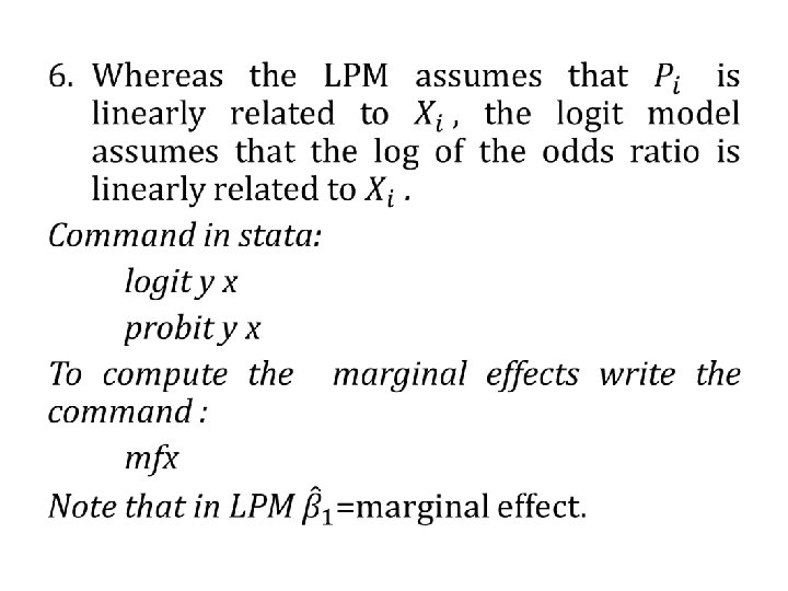
B. Logit and Probit Regression • 2/12/2022 By: Wondimu E. 25

• The CDFs commonly chosen to represent the 0– 1 response models are (1) the logistic and (2) the normal, the former giving rise to the logit model and the latter to the probit (or normit) model. 2/12/2022 By: Wondimu E. 26

i. THE LOGIT MODEL • 2/12/2022 By: Wondimu E. 27

• 2/12/2022 By: Wondimu E. 28

that is, L, the log of the odds ratio, is not only linear in X, but also (from the estimation viewpoint) linear in the parameters. L is called the logit, and hence the name logit model. • Notice these features of the logit model. 1. As P goes from 0 to 1 (i. e. , as Z varies from −∞ to +∞), the logit L goes from −∞ to +∞. That is, although the probabilities (of necessity) lie between 0 and 1, the logits are not so bounded. 2. Although L is linear in X, the probabilities themselves are not. This property is in contrast with the LPM model where the probabilities increase linearly with X. 3. Although we have included only a single X variable, or regressor, in the preceding model, one can add as many regressors as may be dictated by the underlying theory. 2/12/2022 By: Wondimu E. 29

• 2/12/2022 By: Wondimu E. 30

ii. Probit model • 2/12/2022 By: Wondimu E. 32

In binary Regressand models: • 2/12/2022 By: Wondimu E. 33

• 2/12/2022 By: Wondimu E. 34

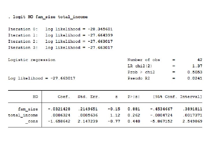
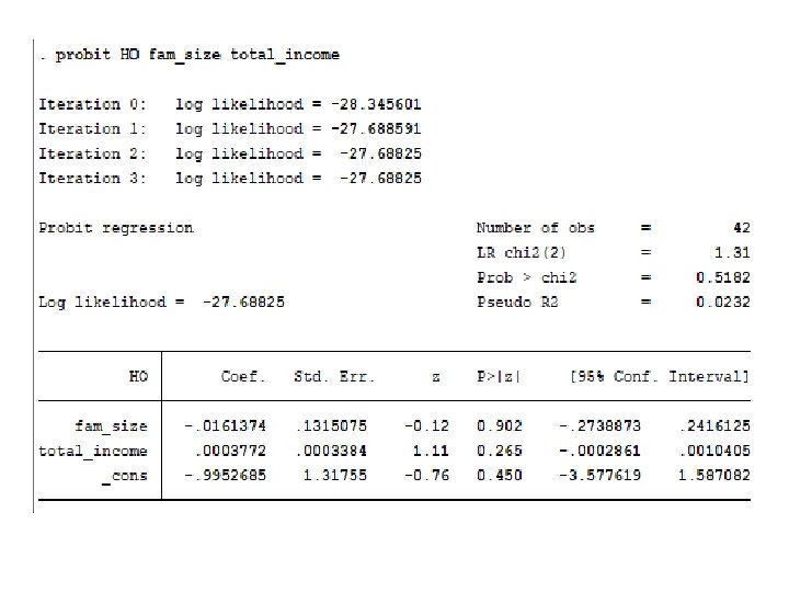
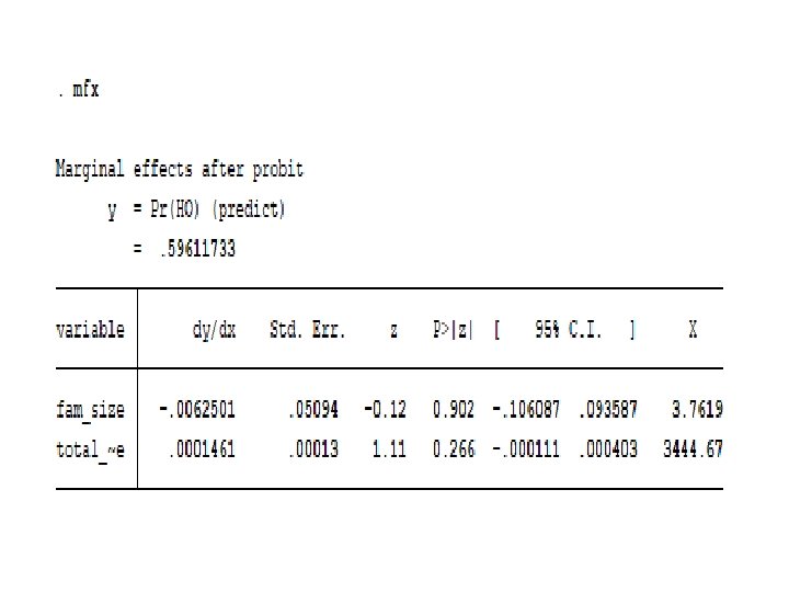
Now compare all the above results of probit, logit and LPM!!!