Panel Regression Panel Data Panel data data that

Panel Regression

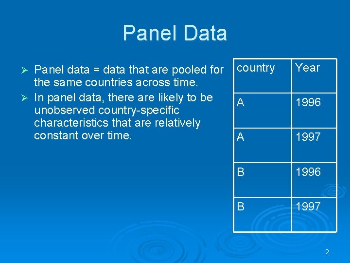
Panel Data Panel data = data that are pooled for the same countries across time. Ø In panel data, there are likely to be unobserved country-specific characteristics that are relatively constant over time. Ø country Year A 1996 A 1997 B 1996 B 1997 2

Advantages of panel regression 3

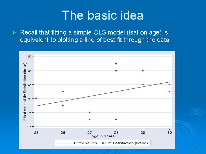
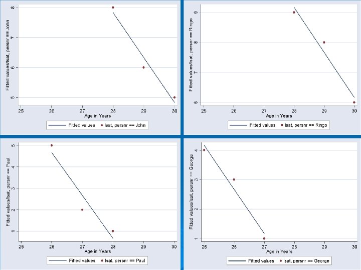
The basic idea Why not OLS (Ordinary Least Squares)? Example The following dataset is a panel of four individuals observed over three years (1968 -70) Ø In each year they were asked how satisfied they are with their lives Ø Ø Ø l Ø this is the lsat variable which takes larger values for increasing satisfaction You want to test how age affects life satisfaction l It appears that they became slightly more satisfied as they got older. 4

The basic idea Ø Recall that fitting a simple OLS model (lsat on age) is equivalent to plotting a line of best fit through the data 5

The basic idea Suppose you now include dummy variables for each individual Ø Recall that you must omit either one dummy variable or the intercept in order to avoid perfect collinearity Ø There now appears to be a highly significant negative impact of age on life satisfaction Ø What’s going on here? Ø 6

7

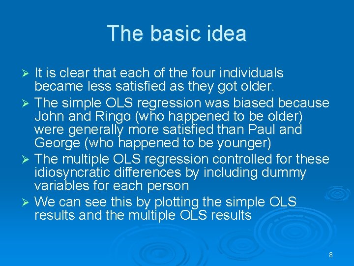
The basic idea It is clear that each of the four individuals became less satisfied as they got older. Ø The simple OLS regression was biased because John and Ringo (who happened to be older) were generally more satisfied than Paul and George (who happened to be younger) Ø The multiple OLS regression controlled for these idiosyncratic differences by including dummy variables for each person Ø We can see this by plotting the simple OLS results and the multiple OLS results Ø 8

9

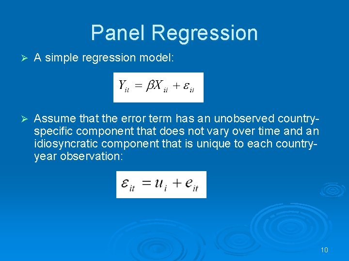
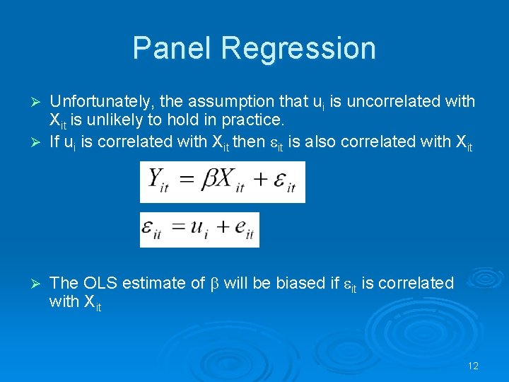
Panel Regression Ø A simple regression model: Ø Assume that the error term has an unobserved countryspecific component that does not vary over time and an idiosyncratic component that is unique to each countryyear observation: 10

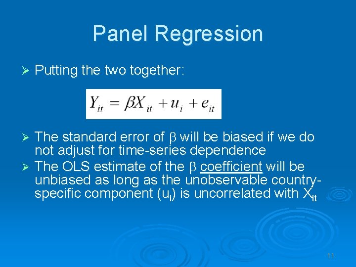
Panel Regression Ø Putting the two together: The standard error of will be biased if we do not adjust for time-series dependence Ø The OLS estimate of the coefficient will be unbiased as long as the unobservable countryspecific component (ui) is uncorrelated with Xit Ø 11

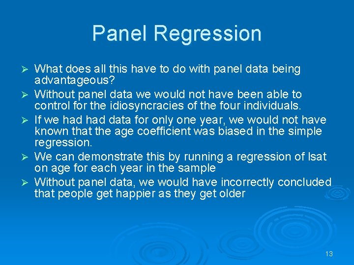
Panel Regression Unfortunately, the assumption that ui is uncorrelated with Xit is unlikely to hold in practice. Ø If ui is correlated with Xit then it is also correlated with Xit Ø Ø The OLS estimate of will be biased if it is correlated with Xit 12

Panel Regression Ø Ø Ø What does all this have to do with panel data being advantageous? Without panel data we would not have been able to control for the idiosyncracies of the four individuals. If we had data for only one year, we would not have known that the age coefficient was biased in the simple regression. We can demonstrate this by running a regression of lsat on age for each year in the sample Without panel data, we would have incorrectly concluded that people get happier as they get older 13

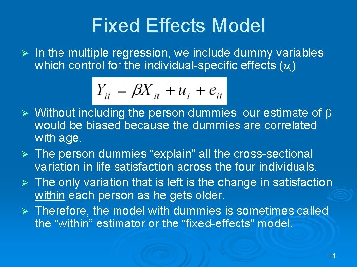
Fixed Effects Model Ø In the multiple regression, we include dummy variables which control for the individual-specific effects (ui) Without including the person dummies, our estimate of would be biased because the dummies are correlated with age. Ø The person dummies “explain” all the cross-sectional variation in life satisfaction across the four individuals. Ø The only variation that is left is the change in satisfaction within each person as he gets older. Ø Therefore, the model with dummies is sometimes called the “within” estimator or the “fixed-effects” model. Ø 14

Fixed Effects Model In small datasets like this, it is easy to create dummy variables for each person (or each country). Ø In large datasets, we may have thousands of individuals or countries. Ø Also it is not very convenient to have results for thousands of dummy variables. Ø 15

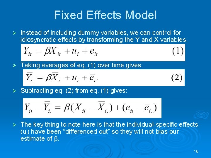
Fixed Effects Model Ø Instead of including dummy variables, we can control for idiosyncratic effects by transforming the Y and X variables. Ø Taking averages of eq. (1) over time gives: Ø Subtracting eq. (2) from eq. (1) gives: Ø The key thing to note here is that the individual-specific effects (ui) have been “differenced out” so they will not bias our estimate of . 16

Fixed effects Ø There are two other issues related with idiosyncratic effects l There may be no such effects • Test redundant fixed effects l These effects may come from some omitted variable(s). 17

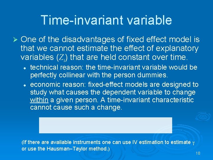
Time-invariant variable Ø One of the disadvantages of fixed effect model is that we cannot estimate the effect of explanatory variables (Zi) that are held constant over time. l l technical reason: the time-invariant variable would be perfectly collinear with the person dummies. economic reason: fixed-effect models are designed to study what causes the dependent variable to change within a given person. A time-invariant characteristic cannot cause such a change. (If there available instruments one can use IV estimation to estimate γ or use the Hausman–Taylor method. ) 18

Random effect model An alternative is the “random effects” model in which the ui are assumed to be randomly distributed with a mean of zero and a constant variance (ui ~ IID(0, 2 u) rather than fixed. Ø Intuitively, the random effects model is like having an OLS model where the intercept varies randomly across individuals i. Ø Like simple OLS, the random effects model assumes that there is zero correlation between ui and Xit Ø If ui and Xit are correlated, the random-effects estimates are biased. Ø 19

Random effect model Ø We can test whether ui and Xit are correlated. l l Ø If they are correlated, we should use the fixed-effects model rather than OLS or the random-effects model (otherwise the coefficients are biased). If they are not correlated, it is better to use the random-effects model (because it is more efficient). The test was devised by Hausman l if ui and Xit are correlated, the random-effects estimates are biased (inconsistent) while the fixed-effects coefficients are unbiased (consistent) • In this case, there will be a large difference between the randomeffects and fixed-effects coefficient estimates l if ui and Xit are uncorrelated, the random-effects and fixed-effects coefficients are both unbiased (consistent); the fixed-effects coefficients are inefficient while the random-effects coefficients are efficient. • In this case, there will not be a large difference between the random -effects and fixed-effects coefficient estimates 20

Random effect model Ø Ø The Hausman test indicates whether the two sets of coefficient estimates are significantly different Null hypothesis (H 0): ui and Xit are uncorrelated The Hausman statistic is distributed as chi 2 If the chi 2 statistic is positive and statistically significant, we can reject the null hypothesis. l Ø This would mean that the fixed-effects model is preferable because the coefficients are consistent. If the chi 2 statistic is not positive and statistically significant, we cannot reject the null hypothesis. l This would mean that the random-effects model is preferable because the coefficients are consistent and efficient. 21

Random effect model If we reject the null hypothesis that ui and Xit are uncorrelated, the fixed-effects model is preferable to the OLS and random-effects models. Ø If we cannot reject the null hypothesis that ui and Xit are uncorrelated, we need to determine whether the ui are distributed randomly across individuals. Ø Random-effects model is like having an OLS model where the constant term varies randomly across individuals i. Ø Therefore, we need to test whethere is significant variation in ui across individuals. Ø 22

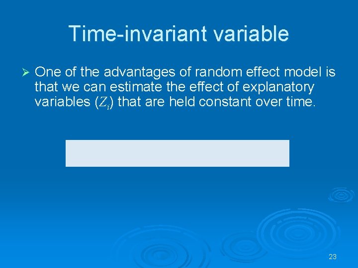
Time-invariant variable Ø One of the advantages of random effect model is that we can estimate the effect of explanatory variables (Zi) that are held constant over time. 23

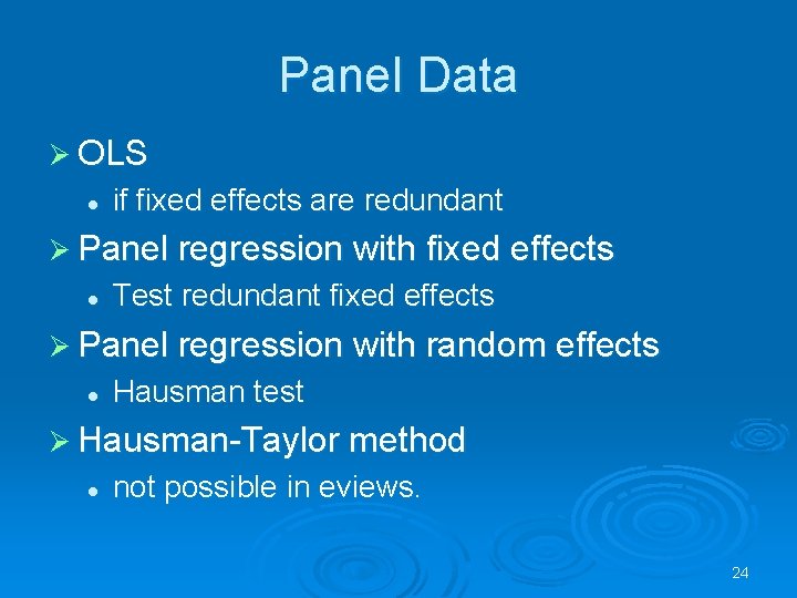
Panel Data Ø OLS l if fixed effects are redundant Ø Panel regression with fixed effects l Test redundant fixed effects Ø Panel regression with random effects l Hausman test Ø Hausman-Taylor method l not possible in eviews. 24