Dimensionality Reduction Chapter 3 Duda et al Section

Dimensionality Reduction Chapter 3 (Duda et al. ) – Section 3. 8 CS 479/679 Pattern Recognition Dr. George Bebis

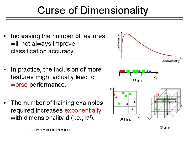
Curse of Dimensionality • Increasing the number of features will not always improve classification accuracy. • In practice, the inclusion of more features might actually lead to worse performance. • The number of training examples required increases exponentially with dimensionality d (i. e. , kd). k: number of bins per feature 31 bins 32 bins 33 bins

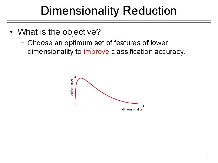
Dimensionality Reduction • What is the objective? − Choose an optimum set of features of lower dimensionality to improve classification accuracy. 3

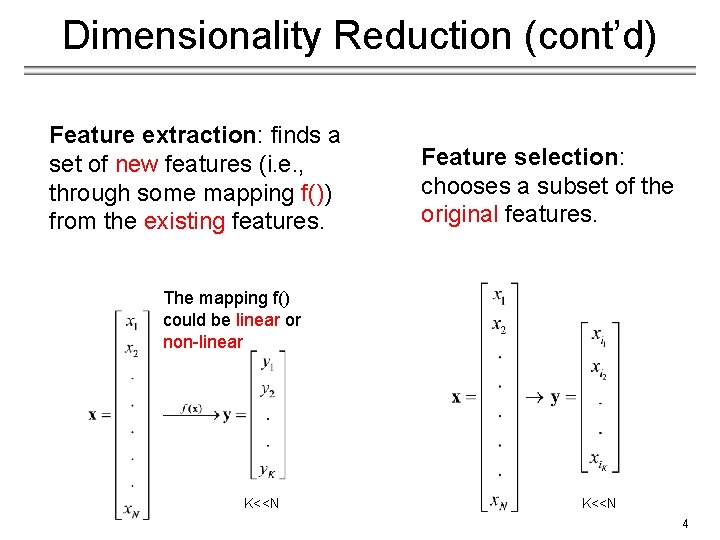
Dimensionality Reduction (cont’d) Feature extraction: finds a set of new features (i. e. , through some mapping f()) from the existing features. Feature selection: chooses a subset of the original features. The mapping f() could be linear or non-linear K<<N 4

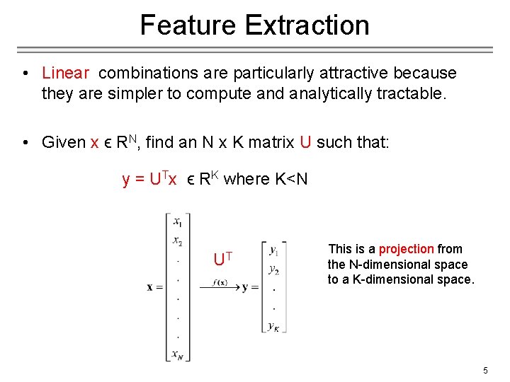
Feature Extraction • Linear combinations are particularly attractive because they are simpler to compute and analytically tractable. • Given x ϵ RN, find an N x K matrix U such that: y = UTx ϵ RK where K<N UT This is a projection from the N-dimensional space to a K-dimensional space. 5

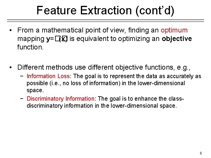
Feature Extraction (cont’d) • From a mathematical point of view, finding an optimum mapping y=�� (x) is equivalent to optimizing an objective function. • Different methods use different objective functions, e. g. , − Information Loss: The goal is to represent the data as accurately as possible (i. e. , no loss of information) in the lower-dimensional space. − Discriminatory Information: The goal is to enhance the classdiscriminatory information in the lower-dimensional space. 6

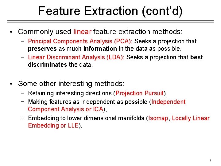
Feature Extraction (cont’d) • Commonly used linear feature extraction methods: − Principal Components Analysis (PCA): Seeks a projection that preserves as much information in the data as possible. − Linear Discriminant Analysis (LDA): Seeks a projection that best discriminates the data. • Some other interesting methods: − Retaining interesting directions (Projection Pursuit), − Making features as independent as possible (Independent Component Analysis or ICA), − Embedding to lower dimensional manifolds (Isomap, Locally Linear Embedding or LLE). 7

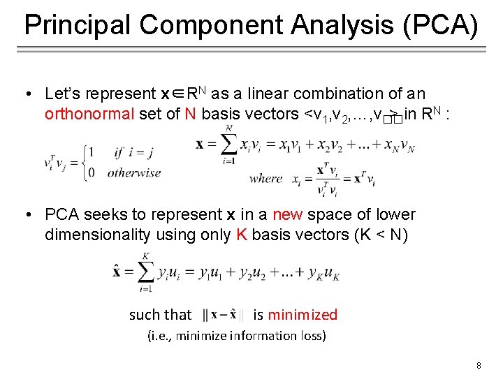
Principal Component Analysis (PCA) • Let’s represent x∈RN as a linear combination of an orthonormal set of N basis vectors <v 1, v 2, …, v�� > in RN : • PCA seeks to represent x in a new space of lower dimensionality using only K basis vectors (K < N) such that is minimized (i. e. , minimize information loss) 8

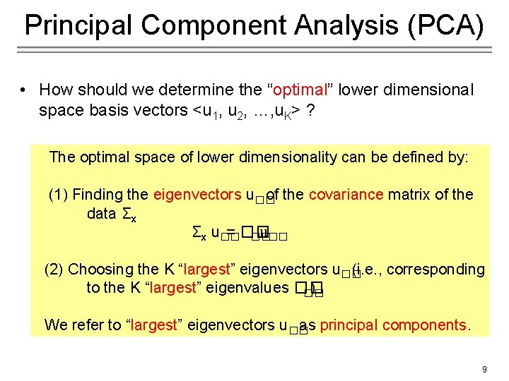
Principal Component Analysis (PCA) • How should we determine the “optimal” lower dimensional space basis vectors <u 1, u 2, …, u. K> ? The optimal space of lower dimensionality can be defined by: (1) Finding the eigenvectors u�� of the covariance matrix of the data Σx Σx u�� = �� u�� �� (2) Choosing the K “largest” eigenvectors u�� (i. e. , corresponding to the K “largest” eigenvalues �� ) �� We refer to “largest” eigenvectors u�� as principal components. 9

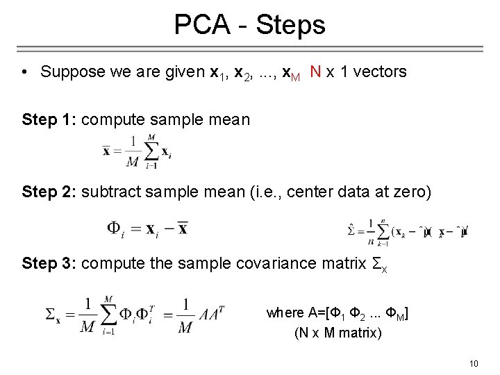
PCA - Steps • Suppose we are given x 1, x 2, . . . , x. M N x 1 vectors Step 1: compute sample mean Step 2: subtract sample mean (i. e. , center data at zero) Step 3: compute the sample covariance matrix Σx where A=[Φ 1 Φ 2. . . ΦΜ] (N x M matrix) 10

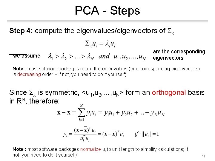
PCA - Steps Step 4: compute the eigenvalues/eigenvectors of Σx we assume are the corresponding eigenvectors Note : most software packages return the eigenvalues (and corresponding eigenvectors) is decreasing order – if not, you need to do it yourself) Since Σx is symmetric, <u 1, u 2, …, u. N> form an orthogonal basis in RN, therefore: Note : most software packages normalize ui to unit length to simplify calculations; if not, you need to do it yourself): 11

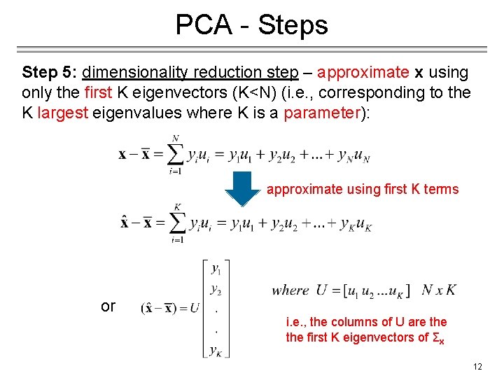
PCA - Steps Step 5: dimensionality reduction step – approximate x using only the first K eigenvectors (K<N) (i. e. , corresponding to the K largest eigenvalues where K is a parameter): approximate using first K terms or i. e. , the columns of U are the first K eigenvectors of Σx 12

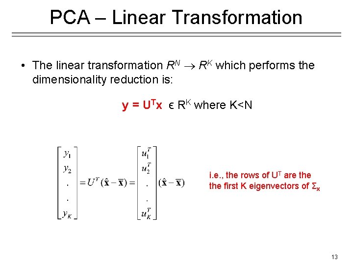
PCA – Linear Transformation • The linear transformation RN RK which performs the dimensionality reduction is: y = UTx ϵ RK where K<N i. e. , the rows of UT are the first K eigenvectors of Σx 13

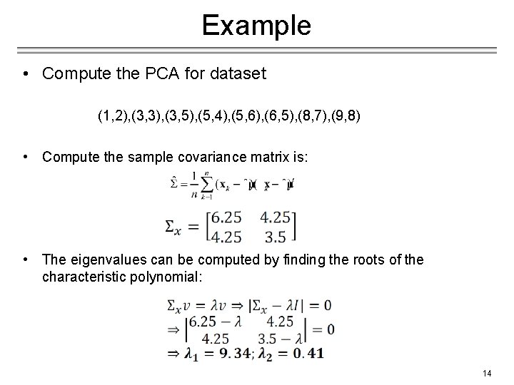
Example • Compute the PCA for dataset (1, 2), (3, 3), (3, 5), (5, 4), (5, 6), (6, 5), (8, 7), (9, 8) • Compute the sample covariance matrix is: • The eigenvalues can be computed by finding the roots of the characteristic polynomial: 14

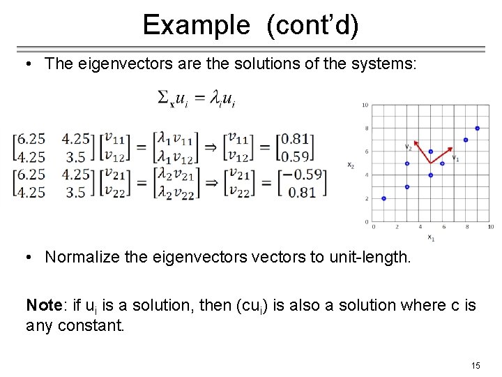
Example (cont’d) • The eigenvectors are the solutions of the systems: • Normalize the eigenvectors to unit-length. Note: if ui is a solution, then (cui) is also a solution where c is any constant. 15

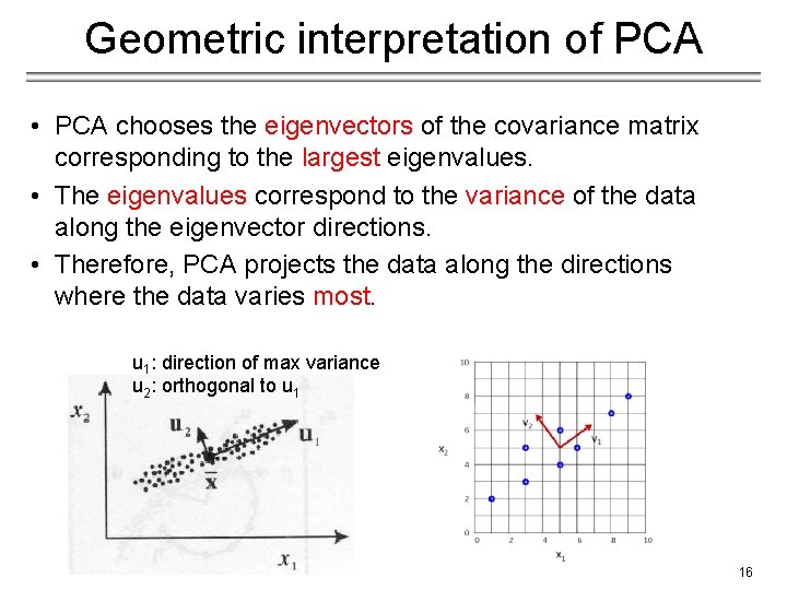
Geometric interpretation of PCA • PCA chooses the eigenvectors of the covariance matrix corresponding to the largest eigenvalues. • The eigenvalues correspond to the variance of the data along the eigenvector directions. • Therefore, PCA projects the data along the directions where the data varies most. u 1: direction of max variance u 2: orthogonal to u 1 16

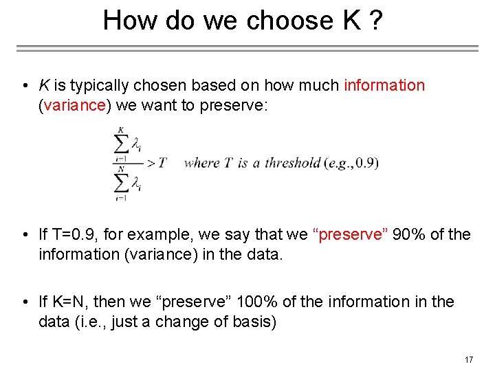
How do we choose K ? • K is typically chosen based on how much information (variance) we want to preserve: • If T=0. 9, for example, we say that we “preserve” 90% of the information (variance) in the data. • If K=N, then we “preserve” 100% of the information in the data (i. e. , just a change of basis) 17

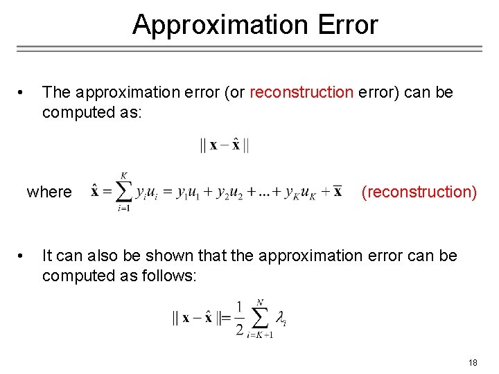
Approximation Error • The approximation error (or reconstruction error) can be computed as: where • (reconstruction) It can also be shown that the approximation error can be computed as follows: 18

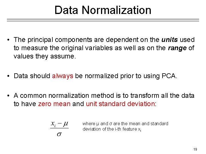
Data Normalization • The principal components are dependent on the units used to measure the original variables as well as on the range of values they assume. • Data should always be normalized prior to using PCA. • A common normalization method is to transform all the data to have zero mean and unit standard deviation: where μ and σ are the mean and standard deviation of the i-th feature xi 19

Comments • PCA simply performs a coordinate rotation that aligns the transformed axes with the directions of maximum variance. • The new covariance matrix Σy is diagonal (i. e. , PCA simply de-correlates the variables). − Note that if the data follow a Gaussian distribution, then the variables also become independent. • The main limitation of PCA is that it does not consider class separability since it does not take into account the class information. − i. e. , there is no guarantee that the directions of maximum variance will contain good features for discrimination. 20

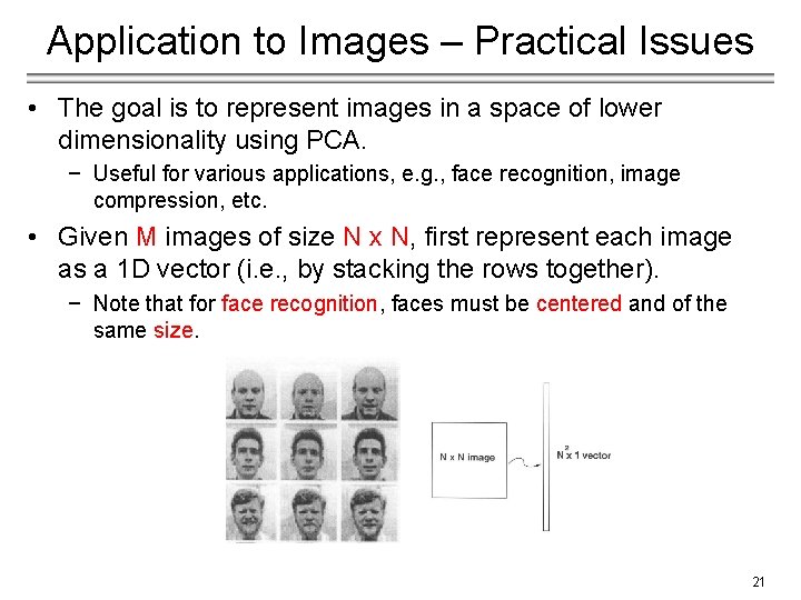
Application to Images – Practical Issues • The goal is to represent images in a space of lower dimensionality using PCA. − Useful for various applications, e. g. , face recognition, image compression, etc. • Given M images of size N x N, first represent each image as a 1 D vector (i. e. , by stacking the rows together). − Note that for face recognition, faces must be centered and of the same size. 21

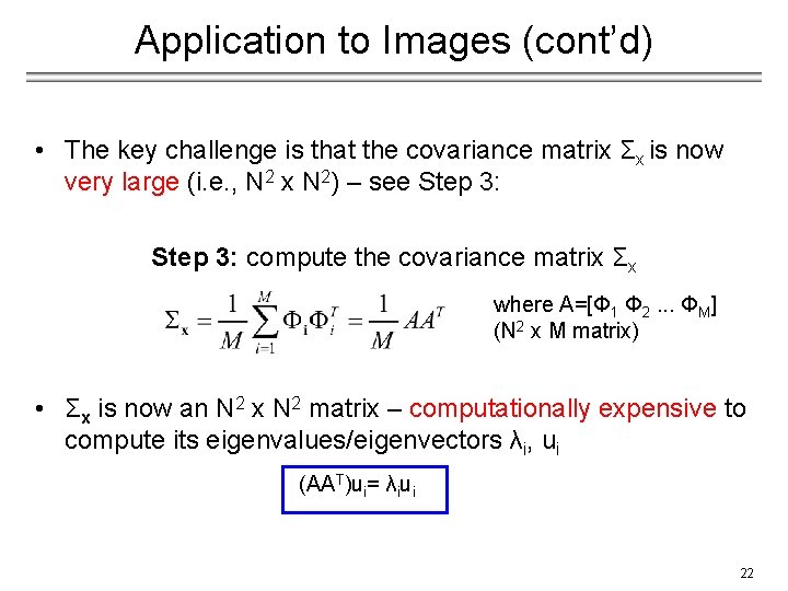
Application to Images (cont’d) • The key challenge is that the covariance matrix Σx is now very large (i. e. , N 2 x N 2) – see Step 3: compute the covariance matrix Σx where A=[Φ 1 Φ 2. . . ΦΜ] (N 2 x M matrix) • Σx is now an N 2 x N 2 matrix – computationally expensive to compute its eigenvalues/eigenvectors λi, ui (AAT)ui= λiui 22

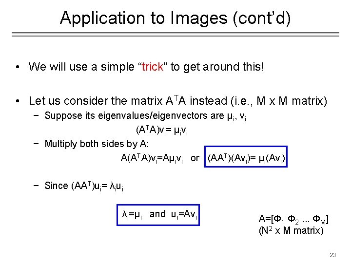
Application to Images (cont’d) • We will use a simple “trick” to get around this! • Let us consider the matrix ATA instead (i. e. , M x M matrix) − Suppose its eigenvalues/eigenvectors are μi, vi (A TA)vi= μivi − Multiply both sides by A: A(ATA)vi=Aμivi or (AAT)(Avi)= μi(Avi) − Since (AAT)ui= λiui λi=μi and ui=Avi A=[Φ 1 Φ 2. . . ΦΜ] (N 2 x M matrix) 23

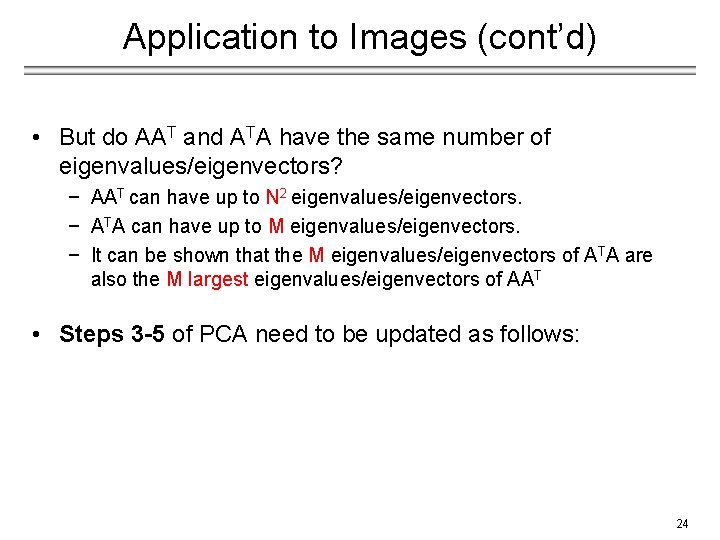
Application to Images (cont’d) • But do AAT and ATA have the same number of eigenvalues/eigenvectors? − AAT can have up to N 2 eigenvalues/eigenvectors. − ATA can have up to M eigenvalues/eigenvectors. − It can be shown that the M eigenvalues/eigenvectors of ATA are also the M largest eigenvalues/eigenvectors of AAT • Steps 3 -5 of PCA need to be updated as follows: 24

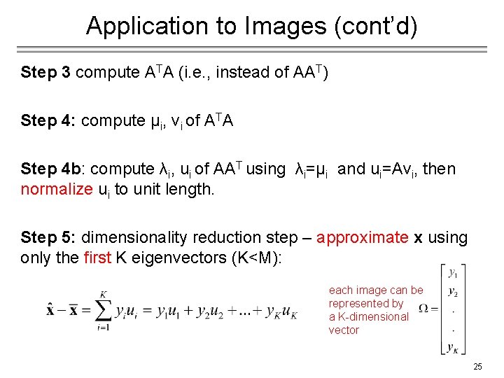
Application to Images (cont’d) Step 3 compute ATA (i. e. , instead of AAT) Step 4: compute μi, vi of ATA Step 4 b: compute λi, ui of AAT using λi=μi and ui=Avi, then normalize ui to unit length. Step 5: dimensionality reduction step – approximate x using only the first K eigenvectors (K<M): each image can be represented by a K-dimensional vector 25

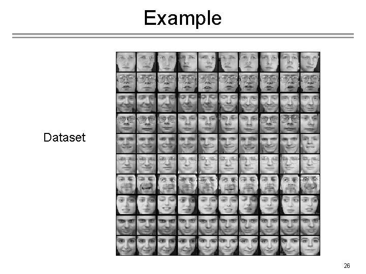
Example Dataset 26

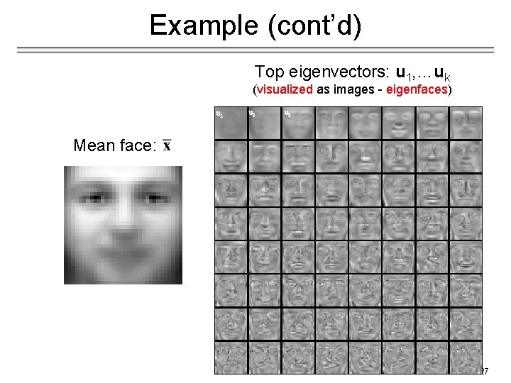
Example (cont’d) Top eigenvectors: u 1, …uk (visualized as images - eigenfaces) u 1 u 2 u 3 Mean face: 27

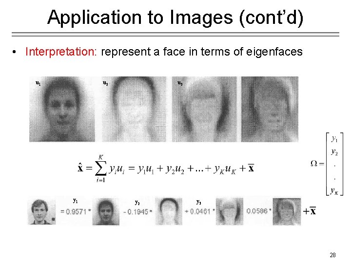
Application to Images (cont’d) • Interpretation: represent a face in terms of eigenfaces u 1 u 2 y 1 u 3 y 2 y 3 28

Case Study: Eigenfaces for Face Detection/Recognition − M. Turk, A. Pentland, "Eigenfaces for Recognition", Journal of Cognitive Neuroscience, vol. 3, no. 1, pp. 71 -86, 1991. • Face Recognition − The simplest approach is to think of it as a template matching problem. − Problems arise when performing recognition in a high-dimensional space. − Use dimensionality reduction! 29

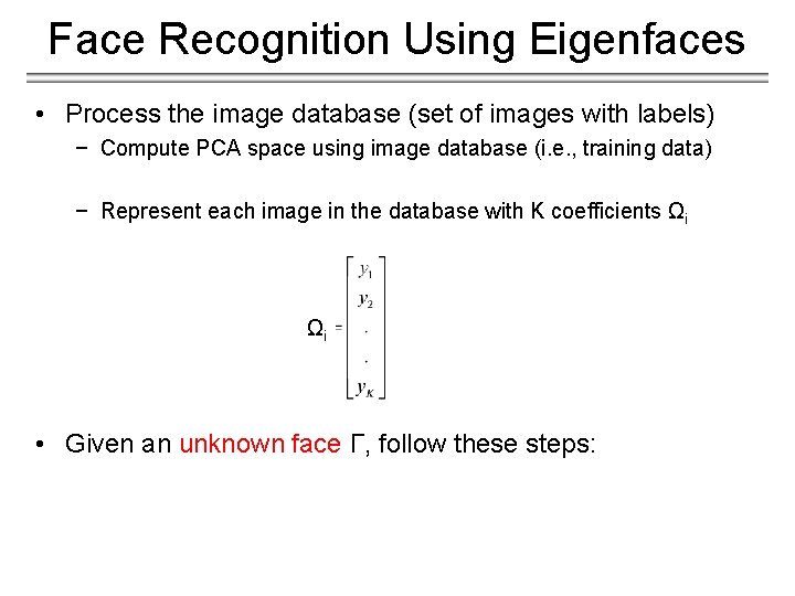
Face Recognition Using Eigenfaces • Process the image database (set of images with labels) − Compute PCA space using image database (i. e. , training data) − Represent each image in the database with K coefficients Ωi Ωi • Given an unknown face Γ, follow these steps:

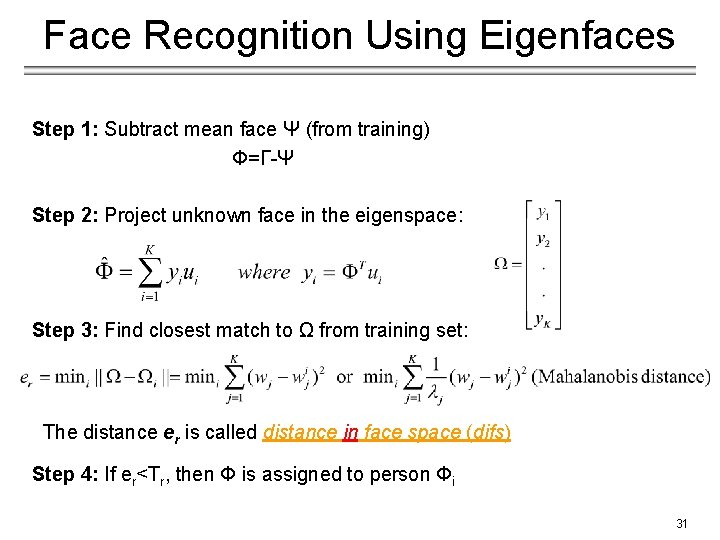
Face Recognition Using Eigenfaces Step 1: Subtract mean face Ψ (from training) Φ=Γ-Ψ Step 2: Project unknown face in the eigenspace: Step 3: Find closest match to Ω from training set: The distance er is called distance in face space (difs) Step 4: If er<Tr, then Φ is assigned to person Φi 31

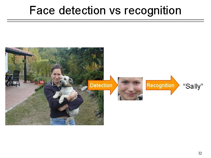
Face detection vs recognition Detection Recognition “Sally” 32

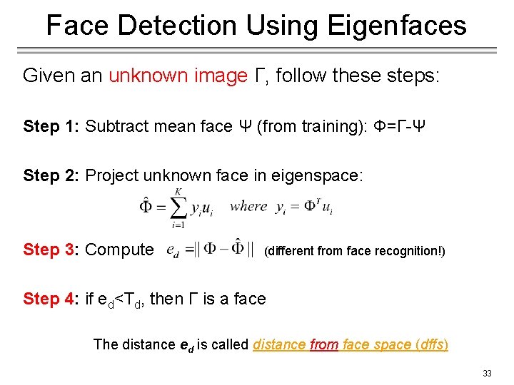
Face Detection Using Eigenfaces Given an unknown image Γ, follow these steps: Step 1: Subtract mean face Ψ (from training): Φ=Γ-Ψ Step 2: Project unknown face in eigenspace: Step 3: Compute (different from face recognition!) Step 4: if ed<Td, then Γ is a face The distance ed is called distance from face space (dffs) 33

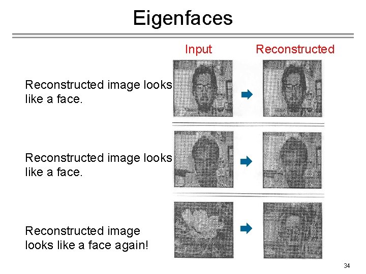
Eigenfaces Input Reconstructed image looks like a face again! 34

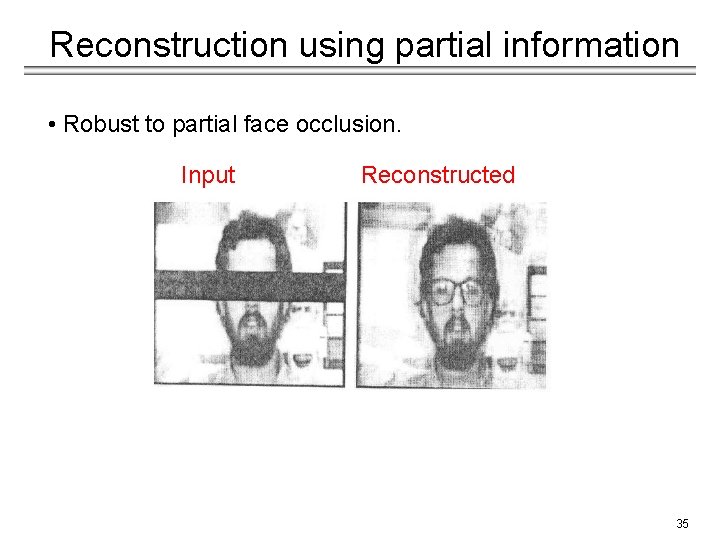
Reconstruction using partial information • Robust to partial face occlusion. Input Reconstructed 35

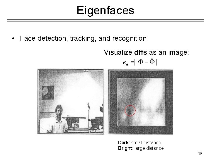
Eigenfaces • Face detection, tracking, and recognition Visualize dffs as an image: Dark: small distance Bright: large distance 36

Limitations • Background changes cause problems − De-emphasize the outside of the face (e. g. , by multiplying the input image by a 2 D Gaussian window centered on the face). • Light changes degrade performance − Light normalization might help but this is a challenging issue. • Performance decreases quickly with changes to face size − Scale input image to multiple sizes. − Multi-scale eigenspaces. • Performance decreases with changes to face orientation (but not as fast as with scale changes) − Out-of-plane rotations are more difficult to handle. − Multi-orientation eigenspaces. 37

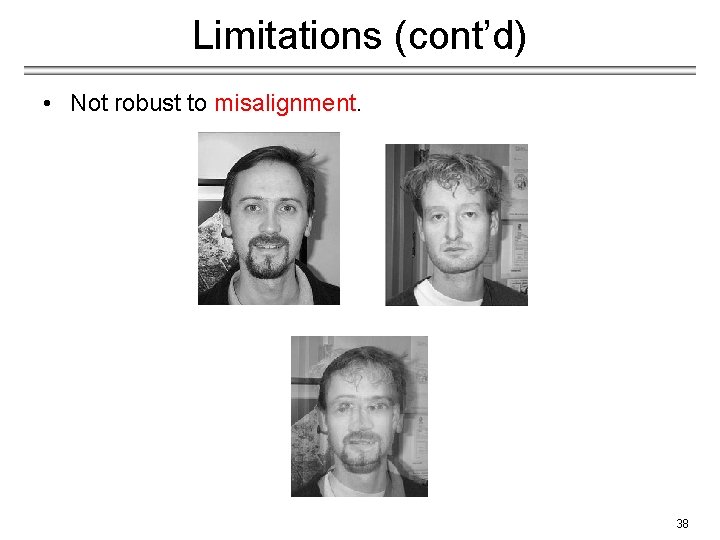
Limitations (cont’d) • Not robust to misalignment. 38

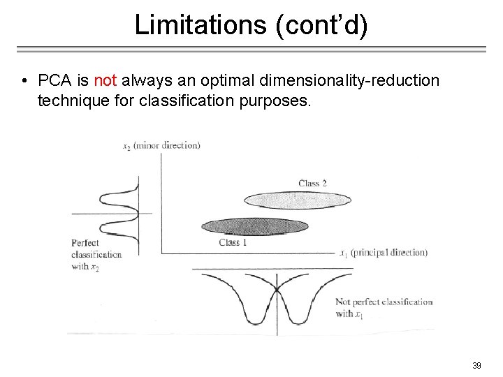
Limitations (cont’d) • PCA is not always an optimal dimensionality-reduction technique for classification purposes. 39

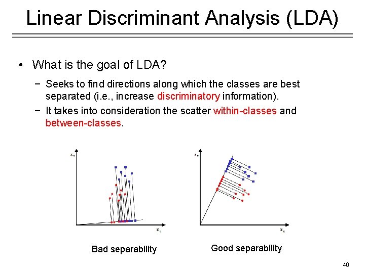
Linear Discriminant Analysis (LDA) • What is the goal of LDA? − Seeks to find directions along which the classes are best separated (i. e. , increase discriminatory information). − It takes into consideration the scatter within-classes and between-classes. Bad separability Good separability 40

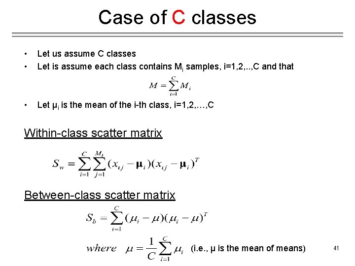
Case of C classes • • Let us assume C classes Let is assume each class contains Mi samples, i=1, 2, . . , C and that • Let μi is the mean of the i-th class, i=1, 2, …, C Within-class scatter matrix Between-class scatter matrix (i. e. , μ is the mean of means) 41

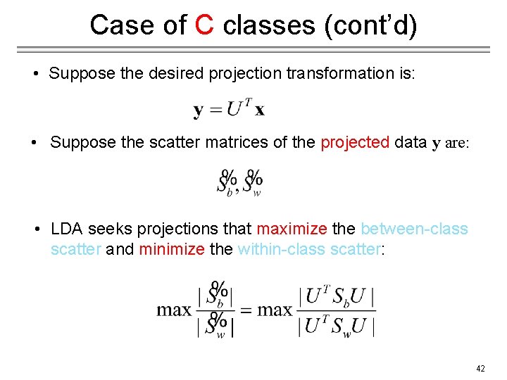
Case of C classes (cont’d) • Suppose the desired projection transformation is: • Suppose the scatter matrices of the projected data y are: • LDA seeks projections that maximize the between-class scatter and minimize the within-class scatter: 42

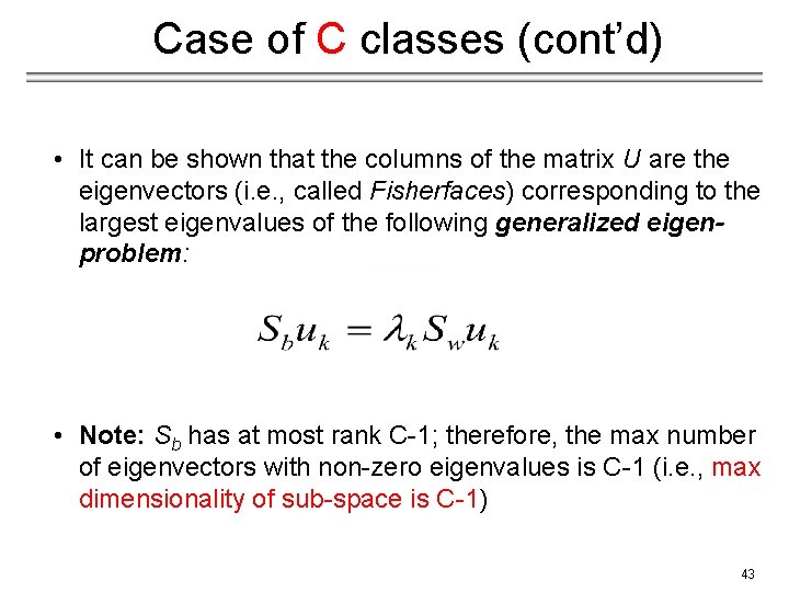
Case of C classes (cont’d) • It can be shown that the columns of the matrix U are the eigenvectors (i. e. , called Fisherfaces) corresponding to the largest eigenvalues of the following generalized eigenproblem: • Note: Sb has at most rank C-1; therefore, the max number of eigenvectors with non-zero eigenvalues is C-1 (i. e. , max dimensionality of sub-space is C-1) 43

Example 44

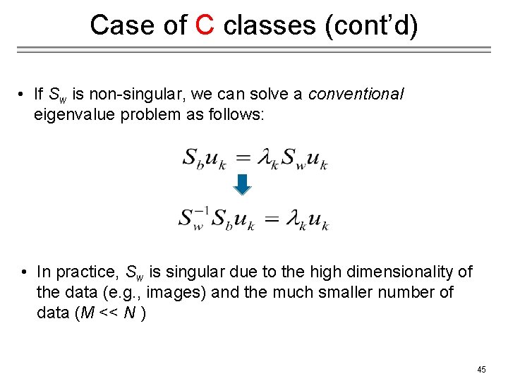
Case of C classes (cont’d) • If Sw is non-singular, we can solve a conventional eigenvalue problem as follows: • In practice, Sw is singular due to the high dimensionality of the data (e. g. , images) and the much smaller number of data (M << N ) 45

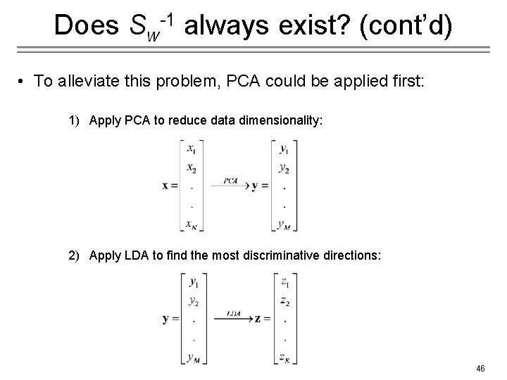
Does Sw-1 always exist? (cont’d) • To alleviate this problem, PCA could be applied first: 1) Apply PCA to reduce data dimensionality: 2) Apply LDA to find the most discriminative directions: 46

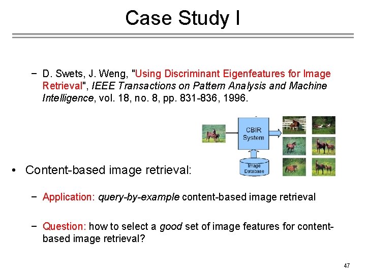
Case Study I − D. Swets, J. Weng, "Using Discriminant Eigenfeatures for Image Retrieval", IEEE Transactions on Pattern Analysis and Machine Intelligence, vol. 18, no. 8, pp. 831 -836, 1996. • Content-based image retrieval: − Application: query-by-example content-based image retrieval − Question: how to select a good set of image features for contentbased image retrieval? 47

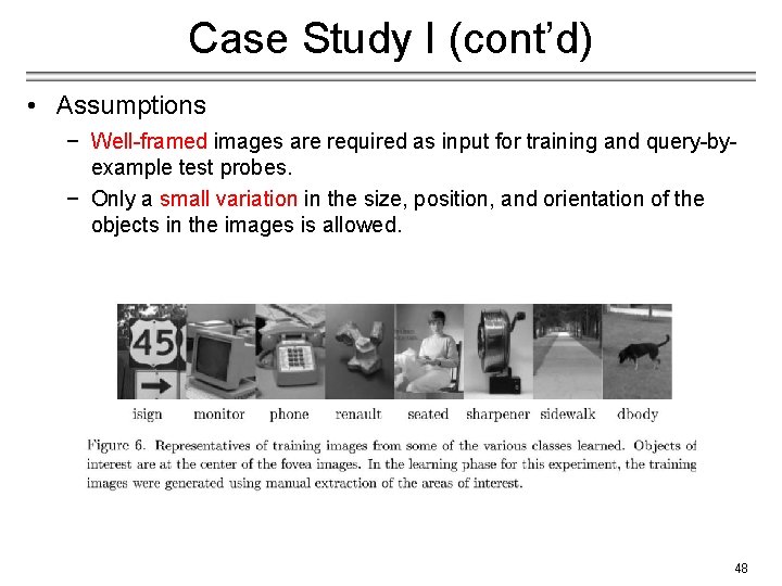
Case Study I (cont’d) • Assumptions − Well-framed images are required as input for training and query-byexample test probes. − Only a small variation in the size, position, and orientation of the objects in the images is allowed. 48

Case Study I (cont’d) • Terminology − Most Expressive Features (MEF): features obtained using PCA. − Most Discriminating Features (MDF): features obtained using LDA. • Numerical instabilities − Computing the eigenvalues/eigenvectors of Sw-1 SBuk = kuk could lead to unstable computations since Sw-1 SB is not always symmetric. − Look in the paper for more details about how to deal with this issue. 49

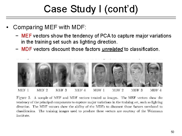
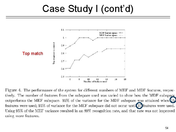
Case Study I (cont’d) • Comparing MEF with MDF: − MEF vectors show the tendency of PCA to capture major variations in the training set such as lighting direction. − MDF vectors discount those factors unrelated to classification. 50

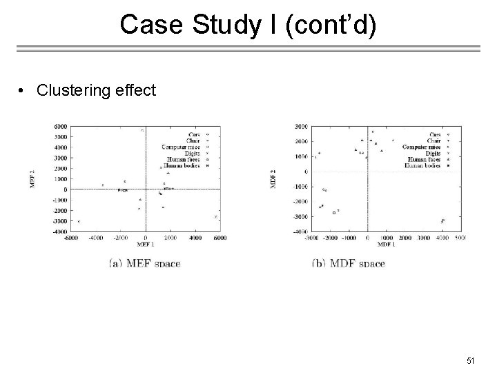
Case Study I (cont’d) • Clustering effect 51

Case Study I (cont’d) • Methodology 1) Represent each training image in terms of MEFs/MDFs. 2) Represent a query image in terms of MEFs/MDFs. 3) Find the k closest neighbors (e. g. , using Euclidean distance). 52

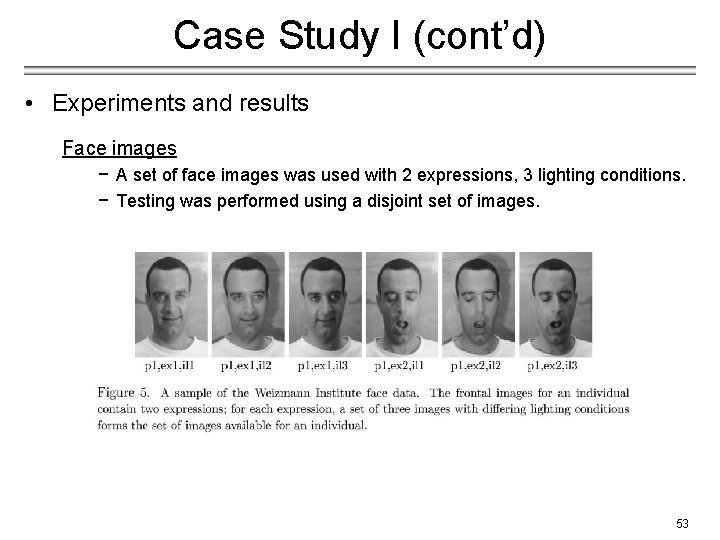
Case Study I (cont’d) • Experiments and results Face images − A set of face images was used with 2 expressions, 3 lighting conditions. − Testing was performed using a disjoint set of images. 53

Case Study I (cont’d) Top match 54

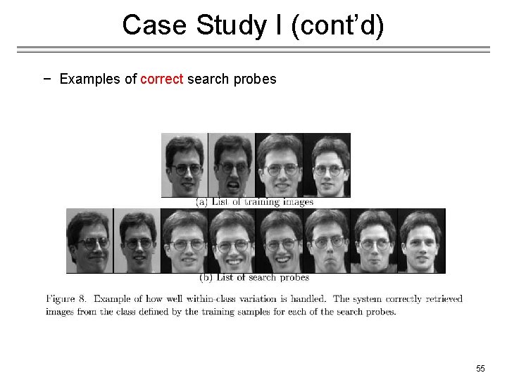
Case Study I (cont’d) − Examples of correct search probes 55

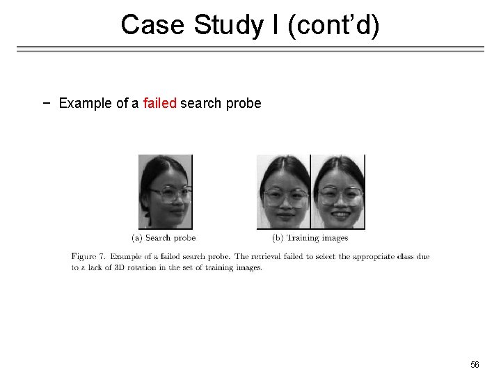
Case Study I (cont’d) − Example of a failed search probe 56

Case Study II − A. Martinez, A. Kak, "PCA versus LDA", IEEE Transactions on Pattern Analysis and Machine Intelligence, vol. 23, no. 2, pp. 228233, 2001. • Is LDA always better than PCA? − There has been a tendency in the computer vision community to prefer LDA over PCA. − This is mainly because LDA deals directly with discrimination between classes while PCA does not pay attention to the underlying class structure. 57

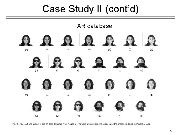
Case Study II (cont’d) AR database 58

Case Study II (cont’d) LDA is not always better when the training set is small 59

Case Study II (cont’d) LDA outperforms PCA when the training set is large 60