Data assimilation shortterm forecast and forecasting error at

Data assimilation, short-term forecast, and forecasting error at convective scales Kao-Shen Chung 鍾高陞 Department of Atmospheric and Oceanic Sciences Mc. Gill University April 19 2010

Outline 1. Introduction 2. Mc. Gill radar assimilation system * impact of the background term 3. Initialization and the short term forecast * case study on 12 July 2004 4. Sensitivity test of the short term forecasts 5. Summary / conclusion 6. Future work

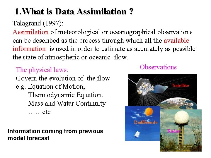
1. What is Data Assimilation ? Talagrand (1997): Assimilation of meteorological or oceanographical observations can be described as the process through which all the available information is used in order to estimate as accurately as possible the state of atmospheric or oceanic flow. Observations The physical laws: Govern the evolution of the flow e. g. Equation of Motion, Thermodynamic Equation, Mass and Water Continuity ……etc Satellite Radiosonde Information coming from previous model forecast Radar

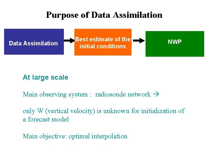
Purpose of Data Assimilation Best estimate of the initial conditions NWP At large scale Main observing system : radiosonde network only W (vertical velocity) is unknown for initialization of a forecast model Main objective: optimal interpolation

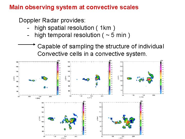
Main observing system at convective scales Doppler Radar provides: - high spatial resolution ( 1 km ) - high temporal resolution ( ~ 5 min ) Capable of sampling the structure of individual Convective cells in a convective system.

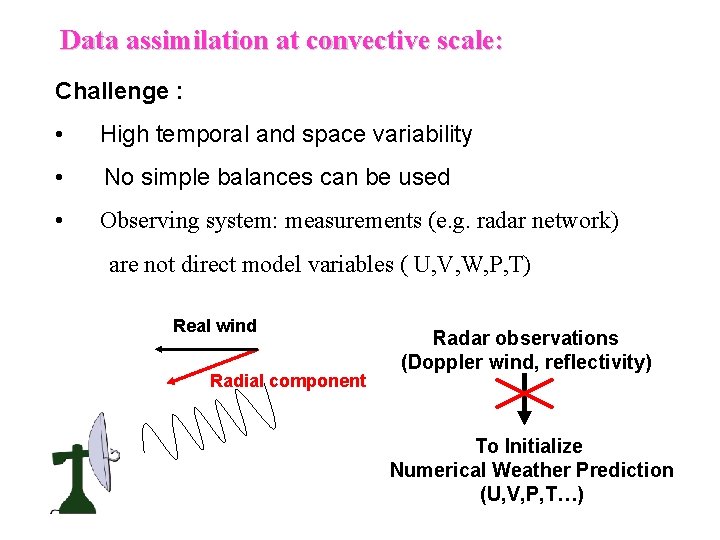
Data assimilation at convective scale: Challenge : • High temporal and space variability • No simple balances can be used • Observing system: measurements (e. g. radar network) are not direct model variables ( U, V, W, P, T) Real wind Radial component Radar observations (Doppler wind, reflectivity) To Initialize Numerical Weather Prediction (U, V, P, T…)

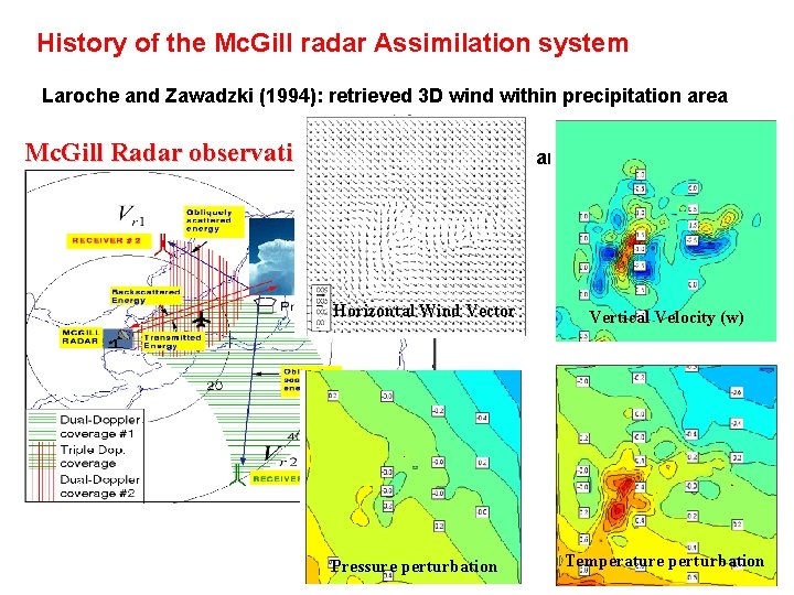
History of the Mc. Gill radar Assimilation system Laroche and Zawadzki (1994): retrieved 3 D wind within precipitation area Mc. Gill Radar observations network Protat and Zawadzki (1999, 2000) Horizontal Wind Vector Pressure perturbation Vertical Velocity (w) Temperature perturbation

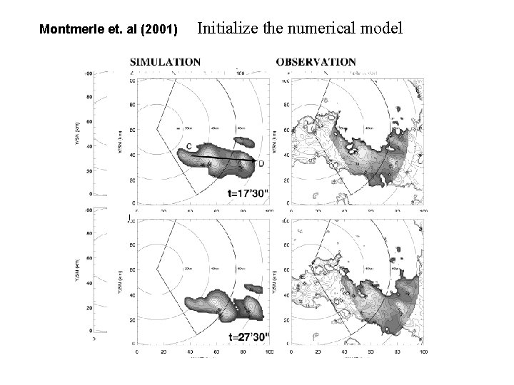
Montmerle et. al (2001) Initialize the numerical model

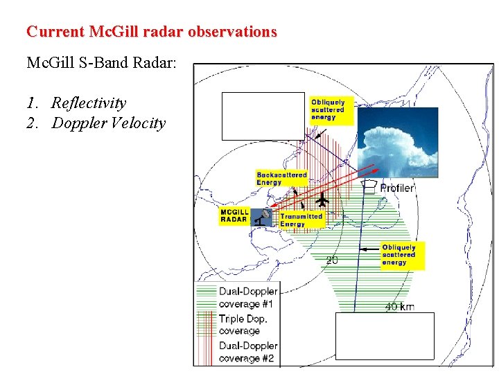
Current Mc. Gill radar observations Mc. Gill S-Band Radar: 1. Reflectivity 2. Doppler Velocity

Challenge and main objective of the research • Observations: single Doppler radar (radial velocity, reflectivity ) • Information other than radar: a prior forecast of a high-resolution model • The predictability / uncertainty of the short term forecast at convective scale

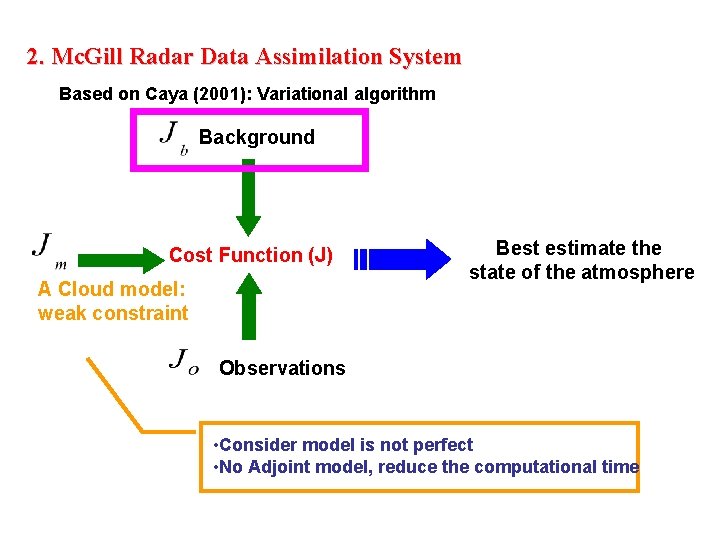
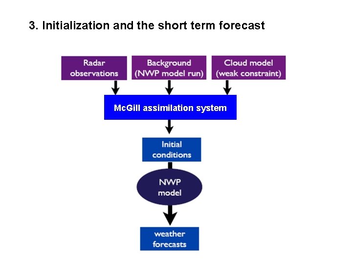
2. Mc. Gill Radar Data Assimilation System Based on Caya (2001): Variational algorithm Background Cost Function (J) A Cloud model: weak constraint Best estimate the state of the atmosphere Observations • Consider model is not perfect • No Adjoint model, reduce the computational time

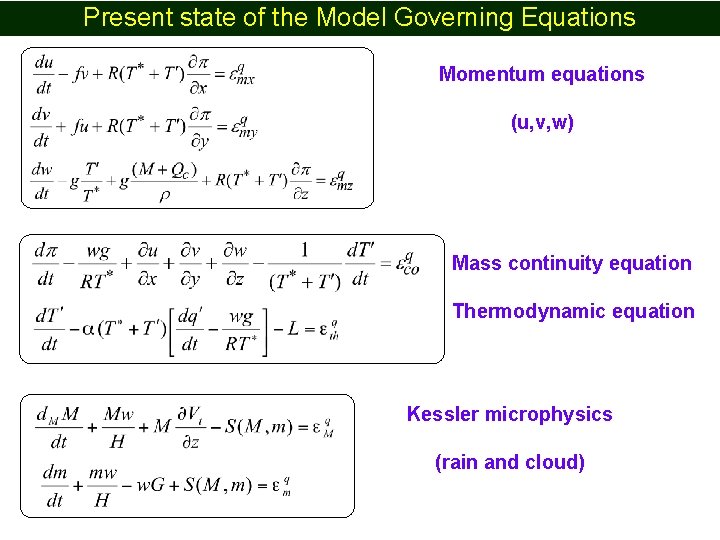
Present state of the Model Governing Equations Momentum equations (u, v, w) Mass continuity equation Thermodynamic equation Kessler microphysics (rain and cloud)

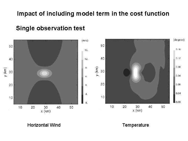
Impact of including model term in the cost function Single observation test Horizontal Wind Temperature

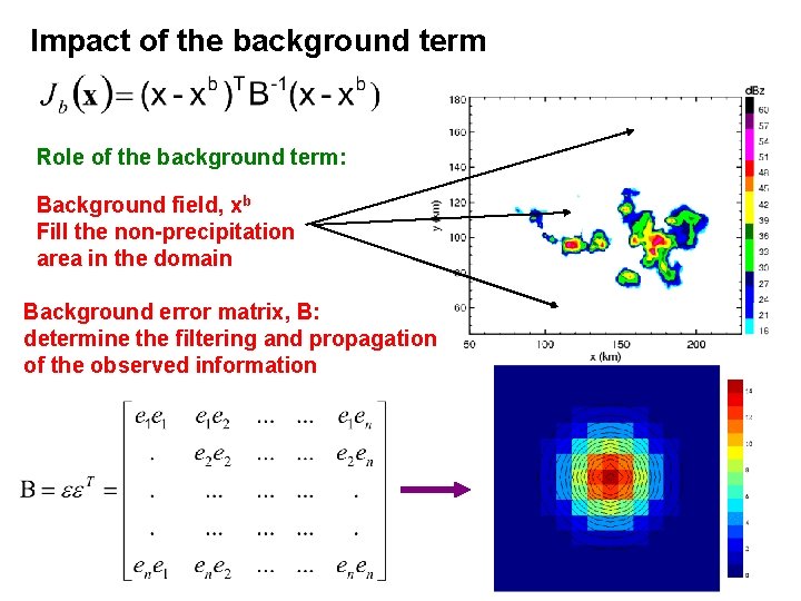
Impact of the background term Role of the background term: Background field, xb Fill the non-precipitation area in the domain Background error matrix, B: determine the filtering and propagation of the observed information

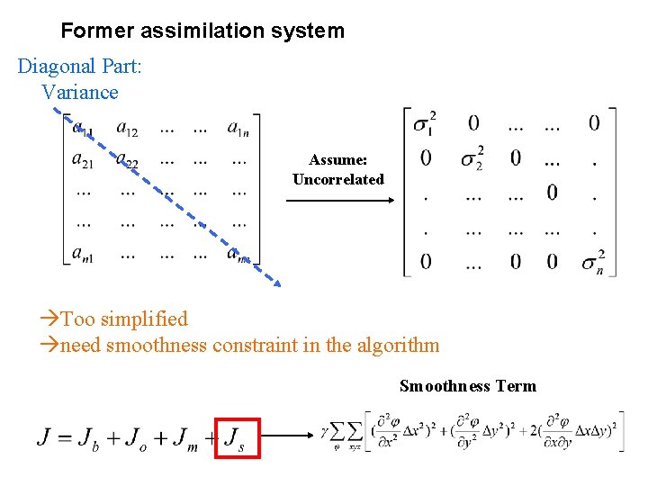
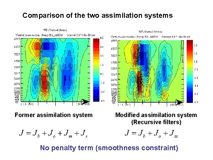
Former assimilation system Diagonal Part: Variance Assume: Uncorrelated Too simplified need smoothness constraint in the algorithm Smoothness Term

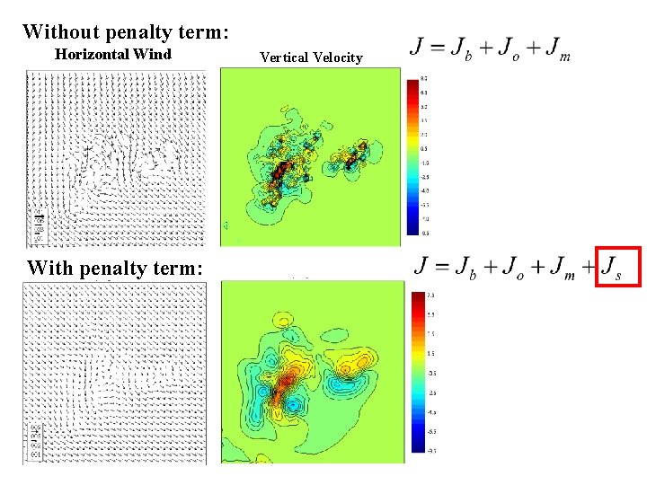
Without penalty term: Horizontal Wind With penalty term: Vertical Velocity

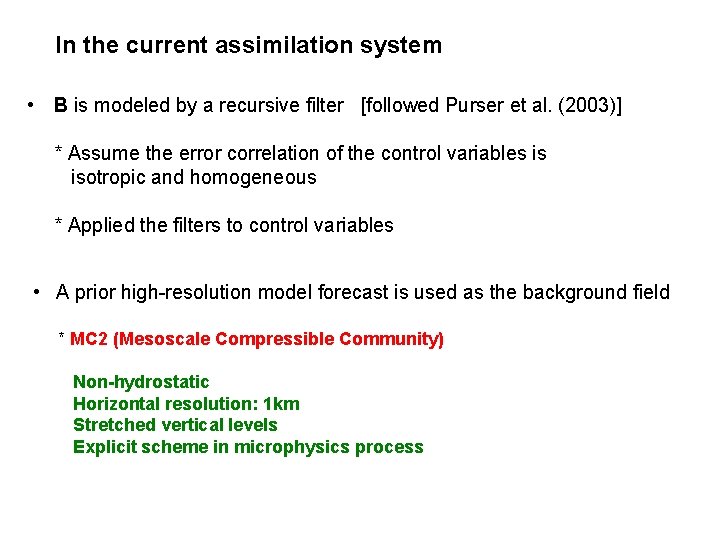
In the current assimilation system • B is modeled by a recursive filter [followed Purser et al. (2003)] * Assume the error correlation of the control variables is isotropic and homogeneous * Applied the filters to control variables • A prior high-resolution model forecast is used as the background field * MC 2 (Mesoscale Compressible Community) Non-hydrostatic Horizontal resolution: 1 km Stretched vertical levels Explicit scheme in microphysics process

Comparison of the two assimilation systems Former assimilation system Modified assimilation system (Recursive filters) No penalty term (smoothness constraint)

3. Initialization and the short term forecast Mc. Gill assimilation system

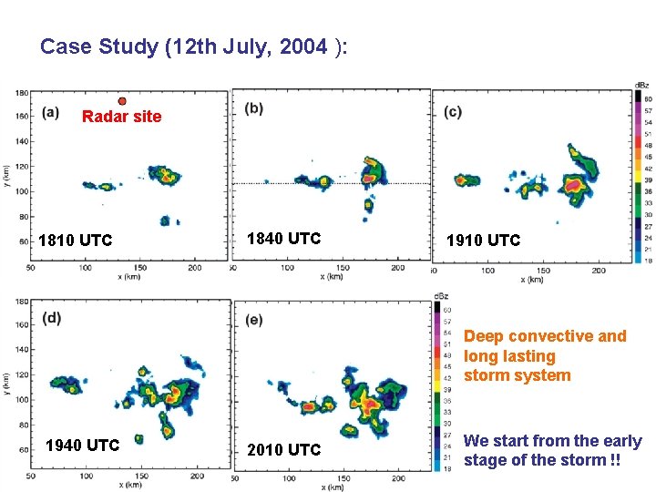
Case Study (12 th July, 2004 ): Radar site 1810 UTC 1840 UTC 1910 UTC Deep convective and long lasting storm system 1940 UTC 2010 UTC We start from the early stage of the storm !!

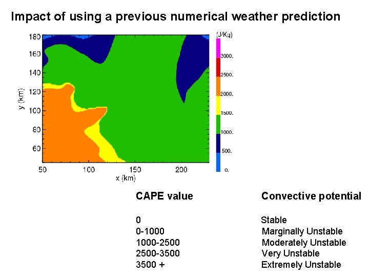
Impact of using a previous numerical weather prediction CAPE value Convective potential 0 0 -1000 -2500 -3500 + Stable Marginally Unstable Moderately Unstable Very Unstable Extremely Unstable

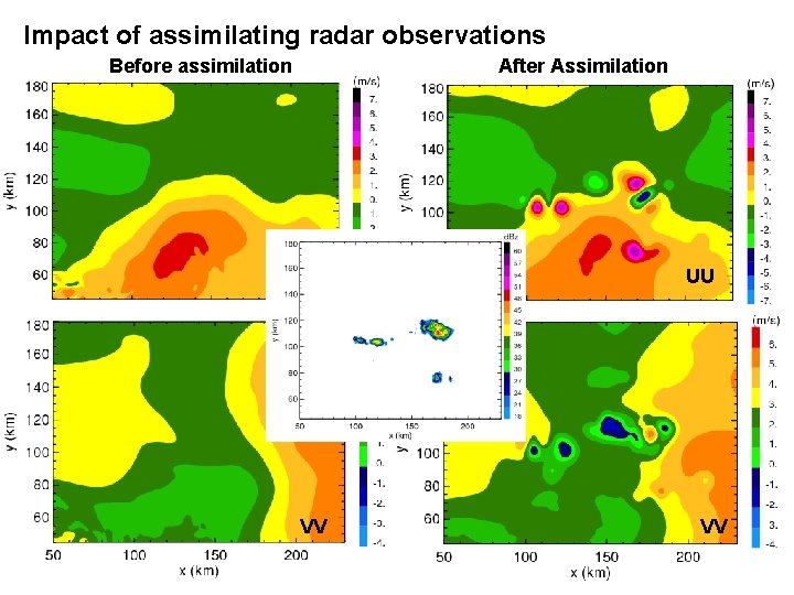
Impact of assimilating radar observations Before assimilation After Assimilation UU VV

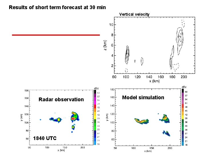
Results of short term forecast at 30 min Vertical velocity Radar observation 1840 UTC Model simulation

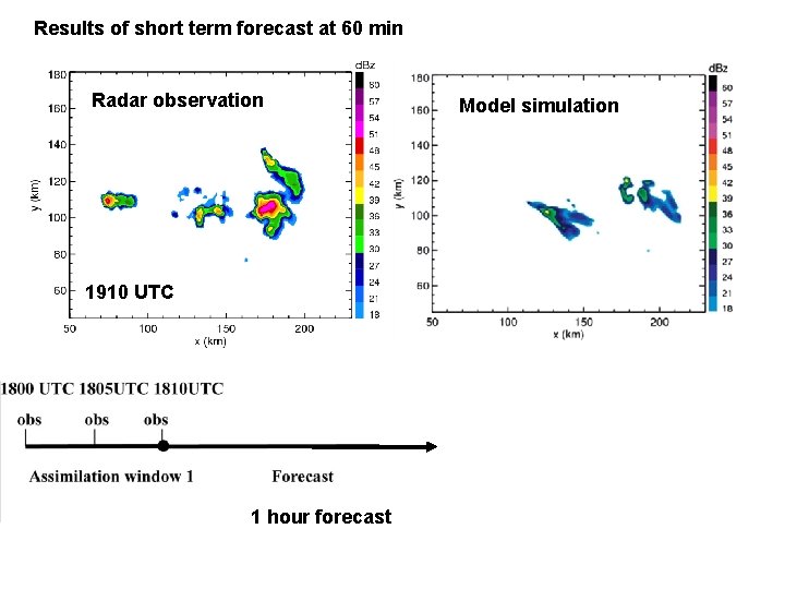
Results of short term forecast at 60 min Radar observation 1910 UTC 1 hour forecast Model simulation

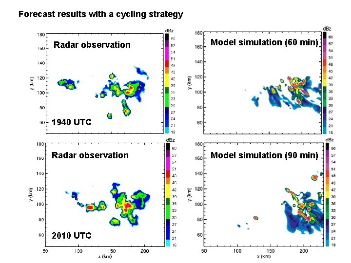
Forecast results with a cycling strategy Radar observation Model simulation (60 min) 1940 UTC Radar observation 2010 UTC Model simulation (90 min)

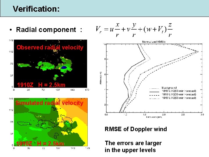
Verification: • Radial component : Observed radial velocity 1910 Z H = 2. 5 km Simulated radial velocity RMSE of Doppler wind 1910 Z H = 2. 5 km The errors are larger in the upper levels

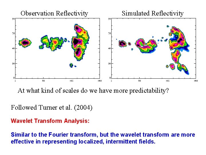
Observation Reflectivity Simulated Reflectivity At what kind of scales do we have more predictability? Followed Turner et al. (2004) Wavelet Transform Analysis: Similar to the Fourier transform, but the wavelet transform are more effective in representing localized, intermittent fields.

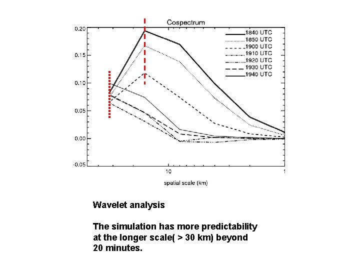
Wavelet analysis The simulation has more predictability at the longer scale( > 30 km) beyond 20 minutes.

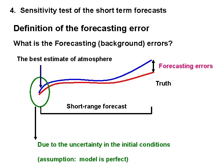
4. Sensitivity test of the short term forecasts Definition of the forecasting error What is the Forecasting (background) errors? The best estimate of atmosphere Forecasting errors Truth Short-range forecast Due to the uncertainty in the initial conditions (assumption: model is perfect)

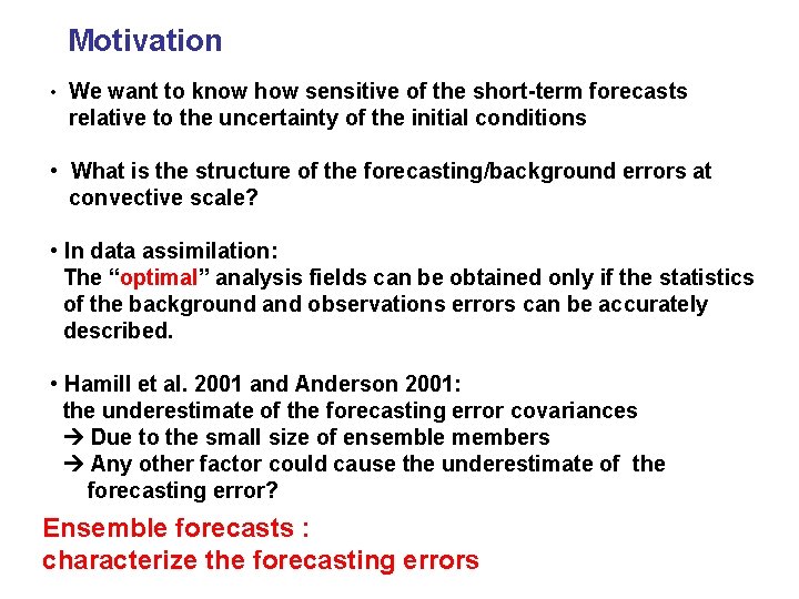
Motivation • We want to know how sensitive of the short-term forecasts relative to the uncertainty of the initial conditions • What is the structure of the forecasting/background errors at convective scale? • In data assimilation: The “optimal” analysis fields can be obtained only if the statistics of the background and observations errors can be accurately described. • Hamill et al. 2001 and Anderson 2001: the underestimate of the forecasting error covariances Due to the small size of ensemble members Any other factor could cause the underestimate of the forecasting error? Ensemble forecasts : characterize the forecasting errors

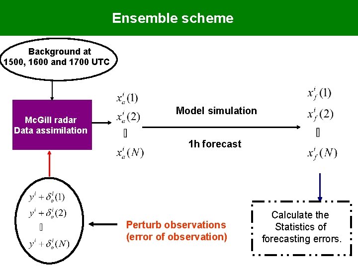
Ensemble scheme Background at 1500, 1600 and 1700 UTC Mc. Gill radar Data assimilation Model simulation 1 h forecast Perturb observations (error of observation) Calculate the Statistics of forecasting errors.

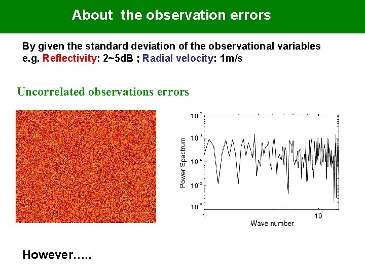
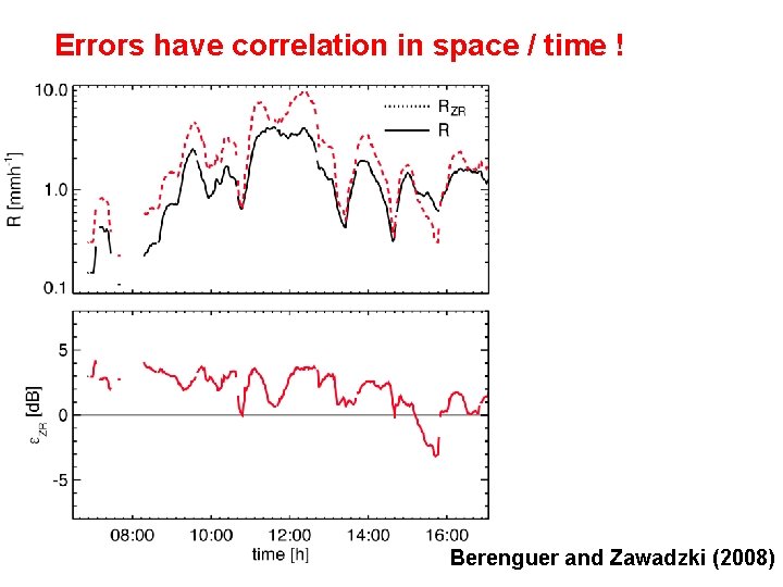
About the observation errors By given the standard deviation of the observational variables e. g. Reflectivity: 2~5 d. B ; Radial velocity: 1 m/s Uncorrelated observations errors However…. .

Errors have correlation in space / time ! Berenguer and Zawadzki (2008)

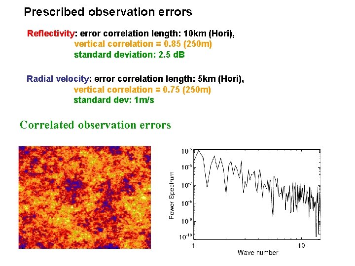
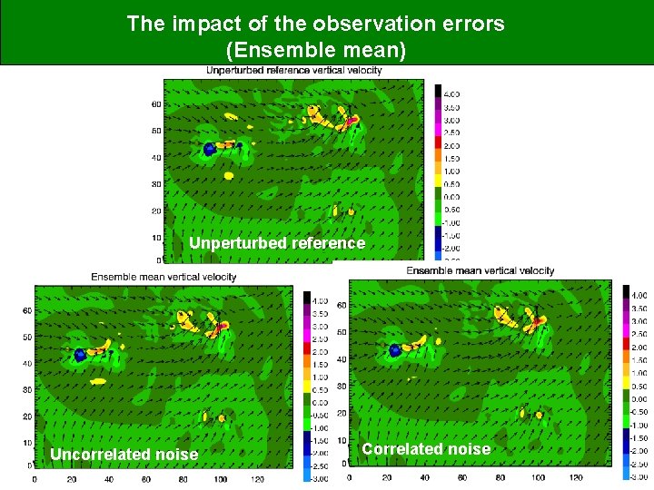
Prescribed observation errors Reflectivity: error correlation length: 10 km (Hori), vertical correlation = 0. 85 (250 m) standard deviation: 2. 5 d. B Radial velocity: error correlation length: 5 km (Hori), vertical correlation = 0. 75 (250 m) standard dev: 1 m/s Correlated observation errors

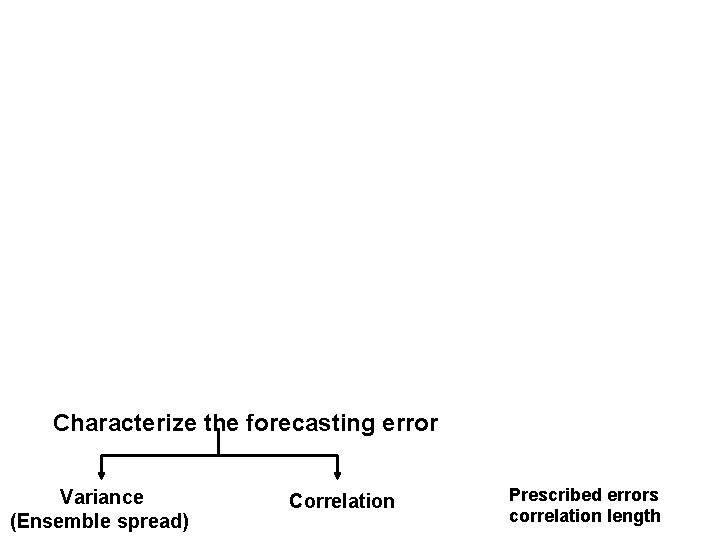
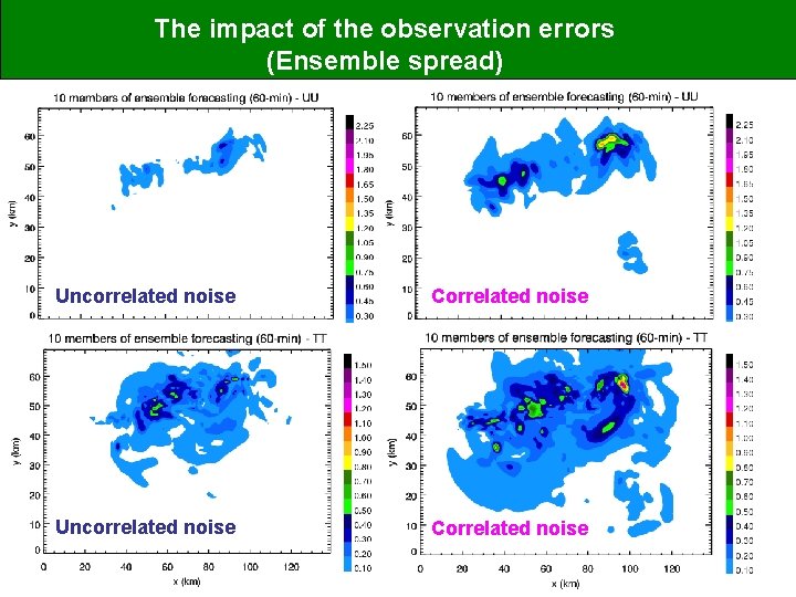
Characterize the forecasting error Variance (Ensemble spread) Correlation Prescribed errors correlation length

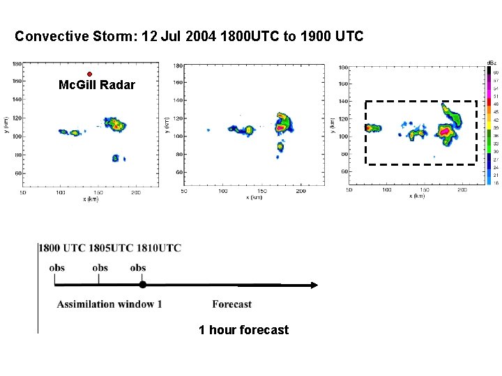
Convective Storm: 12 Jul 2004 1800 UTC to 1900 UTC Mc. Gill Radar 1 hour forecast

The impact of the observation errors (Ensemble mean) Unperturbed reference Uncorrelated noise Correlated noise

The impact of the observation errors (Ensemble spread) Uncorrelated noise Correlated noise

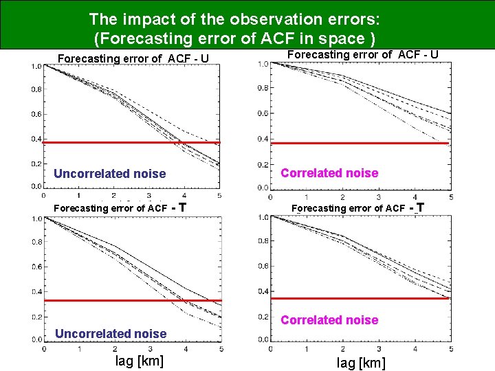
The impact of the observation errors: (Forecasting error of ACF in space ) Forecasting error of ACF - U Correlated noise Uncorrelated noise Forecasting error of ACF Uncorrelated noise lag [km] Forecasting error of ACF - U -T Forecasting error of ACF Correlated noise lag [km] -T

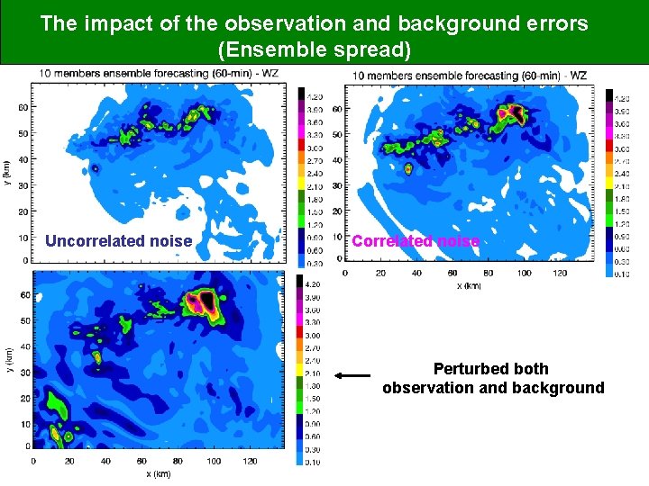
The impact of the observation and background errors (Ensemble spread) Uncorrelated noise Correlated noise Perturbed both observation and background

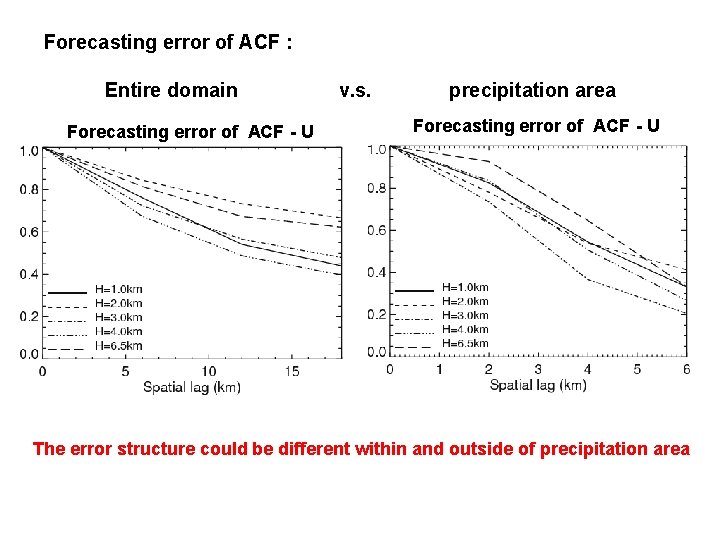
Forecasting error of ACF : Entire domain Forecasting error of ACF - U v. s. precipitation area Forecasting error of ACF - U The error structure could be different within and outside of precipitation area

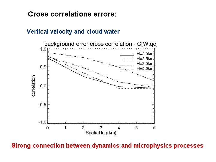
Cross correlations errors: Vertical velocity and cloud water Strong connection between dynamics and microphysics processes

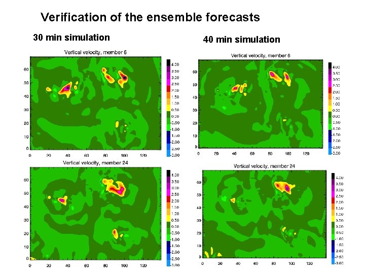
Verification of the ensemble forecasts 30 min simulation 40 min simulation

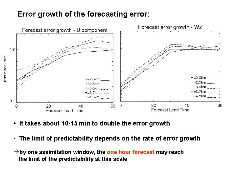
Error growth of the forecasting error: • It takes about 10 -15 min to double the error growth • The limit of predictability depends on the rate of error growth by one assimilation window, the one hour forecast may reach the limit of the predictability at this scale

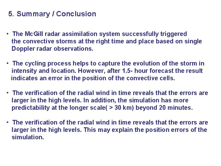
5. Summary / Conclusion • The Mc. Gill radar assimilation system successfully triggered the convective storms at the right time and place based on single Doppler radar observations. • The cycling process helps to capture the evolution of the storm in intensity and location. However, after 1. 5 - hour forecast the result indicates an error in the position of the convective cells. • The verification of the radial wind in time reveals that the errors are larger in the high levels. In addition, the simulation has more predictability at the longer scale( > 30 km) beyond 20 minutes. • The verification of the radial wind in time reveals that the errors are larger in the high levels. This may explain the position errors of the simulation.

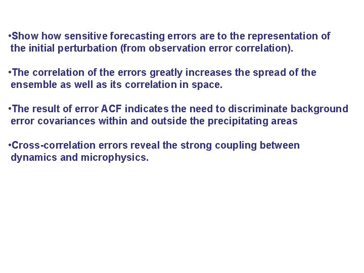
• Show sensitive forecasting errors are to the representation of the initial perturbation (from observation error correlation). • The correlation of the errors greatly increases the spread of the ensemble as well as its correlation in space. • The result of error ACF indicates the need to discriminate background error covariances within and outside the precipitating areas • Cross-correlation errors reveal the strong coupling between dynamics and microphysics.

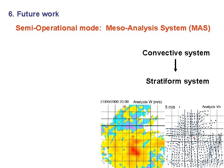
6. Future work Semi-Operational mode: Meso-Analysis System (MAS) Convective system Stratiform system

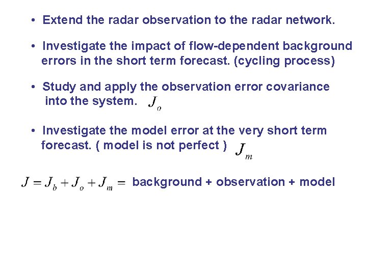
• Extend the radar observation to the radar network. • Investigate the impact of flow-dependent background errors in the short term forecast. (cycling process) • Study and apply the observation error covariance into the system. • Investigate the model error at the very short term forecast. ( model is not perfect ) background + observation + model